Visualizing cross-validation behavior in skada

This example illustrates the use of DA cross-validation object such as DomainShuffleSplit.

Let's prepare the imports:

# Author: Yanis Lalou
#
# License: BSD 3-Clause
# sphinx_gallery_thumbnail_number = 1

import matplotlib.pyplot as plt
import numpy as np
from matplotlib.patches import Patch

from skada.datasets import make_shifted_datasets
from skada.model_selection import (
    DomainShuffleSplit,
    LeaveOneDomainOut,
    SourceTargetShuffleSplit,
    StratifiedDomainShuffleSplit,
)

RANDOM_SEED = 0
cmap_data = plt.cm.PRGn
cmap_domain = plt.cm.RdBu
cmap_cv = plt.cm.coolwarm
n_splits = 4
# Since we'll be using a dataset with 2 source and 2 target domains,
# the lodo splitter will generate only at most 4 splits
n_splits_lodo = 4

First we generate a dataset with 4 different domains. The domains are drawn from 4 different distributions: 2 source and 2 target distributions. The target distributions are shifted versions of the source distributions. Thus we will have a domain adaptation problem with 2 source domains and 2 target domains.

dataset = make_shifted_datasets(
    n_samples_source=3,
    n_samples_target=2,
    shift="conditional_shift",
    label="binary",
    noise=0.4,
    random_state=RANDOM_SEED,
    return_dataset=True,
)

dataset2 = make_shifted_datasets(
    n_samples_source=3,
    n_samples_target=2,
    shift="conditional_shift",
    label="binary",
    noise=0.4,
    random_state=RANDOM_SEED + 1,
    return_dataset=True,
)
dataset.merge(dataset2, names_mapping={"s": "s2", "t": "t2"})

X, y, sample_domain = dataset.pack(
    as_sources=["s", "s2"], as_targets=["t", "t2"], mask_target_labels=True
)
_, target_labels, _ = dataset.pack(
    as_sources=["s", "s2"], as_targets=["t", "t2"], mask_target_labels=False
)

# Sort by sample_domain first then by target_labels
indx_sort = np.lexsort((target_labels, sample_domain))
X = X[indx_sort]
y = y[indx_sort]
target_labels = target_labels[indx_sort]
sample_domain = sample_domain[indx_sort]


# For Lodo methods
X_lodo, y_lodo, sample_domain_lodo = dataset.pack_lodo()

indx_sort = np.lexsort((y_lodo, sample_domain_lodo))
X_lodo = X_lodo[indx_sort]
y_lodo = y_lodo[indx_sort]
sample_domain_lodo = sample_domain_lodo[indx_sort]

We define functions to visualize the behavior of each cross-validation object. The number of splits is set to 4 (2 for the lodo method). For each split, we visualize the indices selected for the training set (in blue) and the test set (in orange).

# Code source: scikit-learn documentation
# Modified for documentation by Yanis Lalou
# License: BSD 3 clause
def plot_cv_indices(cv, X, y, sample_domain, ax, n_splits, lw=10):
    """Create a sample plot for indices of a cross-validation object."""
    # Generate the training/testing visualizations for each CV split
    cv_args = {"X": X, "y": y, "sample_domain": sample_domain}

    for ii, (tr, tt) in enumerate(cv.split(**cv_args)):
        # Fill in indices with the training/test sample_domain
        indices = np.array([np.nan] * len(X))
        indices[tt] = 1
        indices[tr] = 0

        # Visualize the results
        ax.scatter(
            [i / 2 for i in range(1, len(indices) * 2 + 1, 2)],
            [ii + 0.5] * len(indices),
            c=indices,
            marker="_",
            lw=lw,
            cmap=cmap_cv,
            vmin=-0.2,
            vmax=1.2,
        )

    # Plot the data classes and sample_domain at the end
    ax.scatter(
        [i / 2 for i in range(1, len(indices) * 2 + 1, 2)],
        [ii + 1.5] * len(X),
        c=y,
        marker="_",
        lw=lw,
        cmap=cmap_data,
        vmin=-1.2,
        vmax=0.2,
    )

    ax.scatter(
        [i / 2 for i in range(1, len(indices) * 2 + 1, 2)],
        [ii + 2.5] * len(X),
        c=sample_domain,
        marker="_",
        lw=lw,
        cmap=cmap_domain,
        vmin=-3.2,
        vmax=3.2,
    )

    # Formatting
    yticklabels = list(range(n_splits)) + ["class", "sample_domain"]
    ax.set(
        yticks=np.arange(n_splits + 2) + 0.5,
        yticklabels=yticklabels,
        ylim=[n_splits + 2.2, -0.2],
        xlim=[0, len(X)],
    )
    ax.set_title(f"{type(cv).__name__}", fontsize=15)
    return ax


def plot_lodo_indices(cv, X, y, sample_domain, ax, lw=10):
    """Create a sample plot for indices of a cross-validation object."""
    # Generate the training/testing visualizations for each CV split
    cv_args = {"X": X, "y": y, "sample_domain": sample_domain}

    for ii, (tr, tt) in enumerate(cv.split(**cv_args)):
        # Fill in indices with the training/test sample_domain
        indices = np.array([np.nan] * len(X))
        indices[tt] = 1
        indices[tr] = 0

        # Visualize the results
        ax.scatter(
            [i / 2 for i in range(1, len(indices) * 2 + 1, 2)],
            [ii + 0.5] * len(indices),
            c=indices,
            marker="_",
            lw=lw,
            cmap=cmap_cv,
            vmin=-0.2,
            vmax=1.2,
            s=1.8,
        )

    # Plot the data classes and sample_domain at the end
    ax.scatter(
        [i / 2 for i in range(1, len(indices) * 2 + 1, 2)],
        [ii + 1.5] * len(X),
        c=y,
        marker="_",
        lw=lw,
        cmap=cmap_data,
        vmin=-1.2,
        vmax=0.2,
    )

    ax.scatter(
        [i / 2 for i in range(1, len(indices) * 2 + 1, 2)],
        [ii + 2.5] * len(X),
        c=sample_domain,
        marker="_",
        lw=lw,
        cmap=cmap_domain,
        vmin=-3.2,
        vmax=3.2,
    )

    # Formatting
    yticklabels = list(range(n_splits)) + ["class", "sample_domain"]
    ax.set(
        yticks=np.arange(n_splits + 2) + 0.5,
        yticklabels=yticklabels,
        ylim=[n_splits + 2.2, -0.2],
        xlim=[0, len(X)],
    )
    ax.set_title(f"{type(cv).__name__}", fontsize=15)
    return ax


def plot_st_shuffle_indices(cv, X, y, target_labels, sample_domain, ax, n_splits, lw):
    """Create a sample plot for indices of a cross-validation object."""
    for n, labels in enumerate([y, target_labels]):
        # Generate the training/testing visualizations for each CV split
        cv_args = {"X": X, "y": labels, "sample_domain": sample_domain}
        for ii, (tr, tt) in enumerate(cv.split(**cv_args)):
            # Fill in indices with the training/test sample_domain
            indices = np.array([np.nan] * len(X))
            indices[tt] = 1
            indices[tr] = 0

            # Visualize the results
            ax[n].scatter(
                [i / 2 for i in range(1, len(indices) * 2 + 1, 2)],
                [ii + 0.5] * len(indices),
                c=indices,
                marker="_",
                lw=lw,
                cmap=cmap_cv,
                vmin=-0.2,
                vmax=1.2,
            )

        # Plot the data classes and sample_domain at the end
        ax[n].scatter(
            [i / 2 for i in range(1, len(indices) * 2 + 1, 2)],
            [ii + 1.5] * len(X),
            c=labels,
            marker="_",
            lw=lw,
            cmap=cmap_data,
            vmin=-1.2,
            vmax=0.2,
        )

        ax[n].scatter(
            [i / 2 for i in range(1, len(indices) * 2 + 1, 2)],
            [ii + 2.5] * len(X),
            c=sample_domain,
            marker="_",
            lw=lw,
            cmap=cmap_domain,
            vmin=-3.2,
            vmax=3.2,
        )

        # Formatting
        yticklabels = list(range(n_splits)) + ["class", "sample_domain"]
        ax[n].set(
            yticks=np.arange(n_splits + 2) + 0.5,
            yticklabels=yticklabels,
            ylim=[n_splits + 2.2, -0.2],
            xlim=[0, len(X)],
        )

    return ax

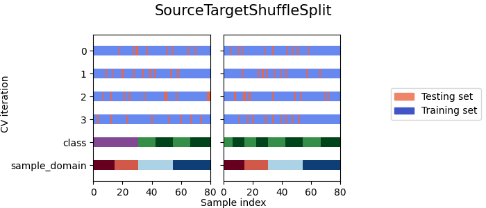
The following plot illustrates the behavior of SourceTargetShuffleSplit. The left plot shows the indices of the training and testing sets for each split and with the datased packed with pack() (the target domains labels are masked (=-1)). While the right plot shows the indices of the training and testing sets for each split and with the datased packed with pack() and argument mask_target_labels=False

cvs = [SourceTargetShuffleSplit]
for cv in cvs:
    fig, ax = plt.subplots(1, 2, figsize=(7, 3), sharey=True)
    fig.suptitle(f"{cv.__name__}", fontsize=15)
    plot_st_shuffle_indices(
        cv(n_splits), X, y, target_labels, sample_domain, ax, n_splits, 10
    )

    fig.legend(
        [Patch(color=cmap_cv(0.8)), Patch(color=cmap_cv(0.02))],
        ["Testing set", "Training set"],
        loc="center right",
    )
    fig.text(0.48, 0.01, "Sample index", ha="center")
    fig.text(0.001, 0.5, "CV iteration", va="center", rotation="vertical")

    # Make the legend fit
    plt.tight_layout()
    fig.subplots_adjust(right=0.7)

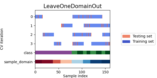
The following plot illustrates the behavior of LeaveOneDomainOut. The plot shows the indices of the training and testing sets for each split and which domain is used as the target domain for each split.

cvs = [LeaveOneDomainOut]
for cv in cvs:
    fig, ax = plt.subplots(figsize=(6, 3))
    plot_lodo_indices(cv(n_splits_lodo), X_lodo, y_lodo, sample_domain_lodo, ax)

    fig.legend(
        [Patch(color=cmap_cv(0.8)), Patch(color=cmap_cv(0.02))],
        ["Testing set", "Training set"],
        loc="center right",
    )
    fig.text(0.48, 0.01, "Sample index", ha="center")
    fig.text(0.001, 0.5, "CV iteration", va="center", rotation="vertical")

    # Make the legend fit
    plt.tight_layout()
    fig.subplots_adjust(right=0.7)

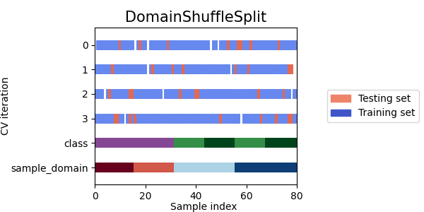
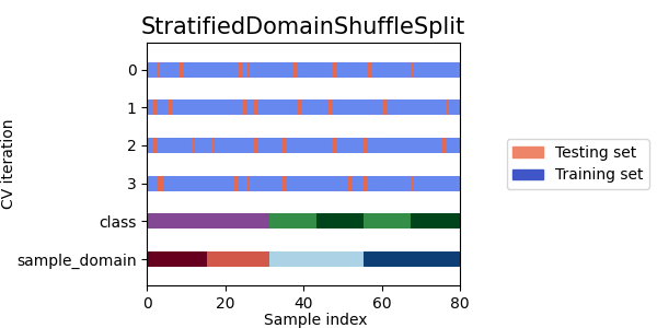
Now let's see how the other cross-validation objects behave on our dataset.

cvs = [
    DomainShuffleSplit,
    StratifiedDomainShuffleSplit,
]

for cv in cvs:
    fig, ax = plt.subplots(figsize=(6, 3))
    plot_cv_indices(cv(n_splits), X, y, sample_domain, ax, n_splits)

    fig.legend(
        [Patch(color=cmap_cv(0.8)), Patch(color=cmap_cv(0.02))],
        ["Testing set", "Training set"],
        loc="center right",
    )
    fig.text(0.48, 0.01, "Sample index", ha="center")
    fig.text(0.001, 0.5, "CV iteration", va="center", rotation="vertical")

    # Make the legend fit
    plt.tight_layout()
    fig.subplots_adjust(right=0.7)

• 
• 

As we can see each splitter has a very different behavior:

• SourceTargetShuffleSplit: Each sample is used once as a test set while the remaining samples form the training set.

• DomainShuffleSplit: Randomly split the data depending on their sample_domain. Each fold is composed of samples coming from all source and target domains.

• StratifiedDomainShuffleSplit: Same as DomainShuffleSplit but by also preserving the percentage of samples for each class and for each sample domain. Split depends not only on the samples sample_domain but also their label.

• LeaveOneDomainOut: Each sample with the same sample_domain is used once as the target domain, while the remaining samples from the others sample_domain for the source domain (Can be used only with pack_lodo())