Gradual Domain Adaptation Using Optimal Transport

This example illustrates the GOAT method from [38] on a simple classification task. However, the CNN is replaced with a MLP.

[38]

Y. He, H. Wang, B. Li, H. Zhao Gradual Domain Adaptation: Theory and Algorithms in Journal of Machine Learning Research, 2024.

# Authors: Félix Lefebvre and Julie Alberge
#
# License: BSD 3-Clause

import matplotlib.pyplot as plt
from sklearn.inspection import DecisionBoundaryDisplay
from sklearn.neural_network import MLPClassifier

from skada import source_target_split
from skada._gradual_da import GradualEstimator
from skada.datasets import make_shifted_datasets

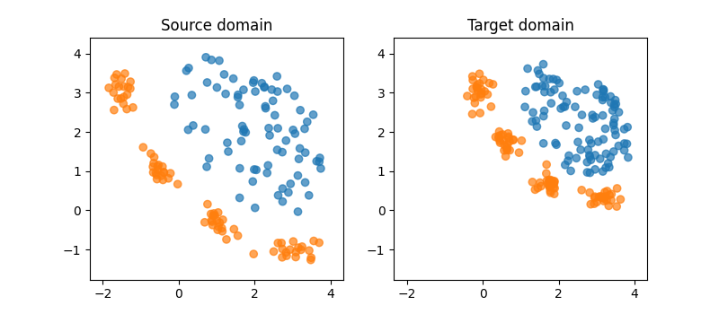
Generate conditional shift dataset

n, m = 20, 25  # number of source and target samples
X, y, sample_domain = make_shifted_datasets(
    n_samples_source=n,
    n_samples_target=m,
    shift="conditional_shift",
    noise=0.1,
    random_state=42,
)

Plot source and target datasets

X_source, X_target, y_source, y_target = source_target_split(
    X, y, sample_domain=sample_domain
)
lims = (min(X[:, 0]) - 0.5, max(X[:, 0]) + 0.5, min(X[:, 1]) - 0.5, max(X[:, 1]) + 0.5)

n_tot_source = X_source.shape[0]
n_tot_target = X_target.shape[0]

plt.figure(1, figsize=(8, 3.5))
plt.subplot(121)

plt.scatter(X_source[:, 0], X_source[:, 1], c=y_source, vmax=9, cmap="tab10", alpha=0.7)
plt.title("Source domain")
plt.axis(lims)

plt.subplot(122)
plt.scatter(X_target[:, 0], X_target[:, 1], c=y_target, vmax=9, cmap="tab10", alpha=0.7)
plt.title("Target domain")
plt.axis(lims)

(np.float64(-2.3407051687007465), np.float64(4.329230428885397), np.float64(-1.765584745112177), np.float64(4.406935559355198))

Fit Gradual Domain Adaptation

We use a MLP classifier as the base estimator (default parameters).

base_estimator = MLPClassifier(hidden_layer_sizes=(50, 50))

gradual_adapter = GradualEstimator(
    n_steps=40,  # number of adaptation steps
    base_estimator=base_estimator,
    advanced_ot_plan_sampling=True,
    save_estimators=True,
    save_intermediate_data=True,
)

gradual_adapter.fit(
    X,
    y,
    sample_domain=sample_domain,
)

/home/circleci/.local/lib/python3.10/site-packages/sklearn/neural_network/_multilayer_perceptron.py:781: ConvergenceWarning: Stochastic Optimizer: Maximum iterations (200) reached and the optimization hasn't converged yet.
  warnings.warn(

GradualEstimator(advanced_ot_plan_sampling=True,
                 base_estimator=MLPClassifier(hidden_layer_sizes=(50, 50),
                                              max_iter=4200),
                 n_steps=40, save_estimators=True, save_intermediate_data=True)

In a Jupyter environment, please rerun this cell to show the HTML representation or trust the notebook.
On GitHub, the HTML representation is unable to render, please try loading this page with nbviewer.org.

Check results

Compute accuracy on source and target with the initial estimator and the final estimator.

clfs = gradual_adapter.get_intermediate_estimators()

ACC_source_init = clfs[0].score(X_source, y_source)
ACC_target_init = clfs[0].score(X_target, y_target)

print(f"Initial accuracy on source domain: {ACC_source_init:.3f}")
print(f"Initial accuracy on target domain: {ACC_target_init:.3f}")
print("")

ACC_source = gradual_adapter.score(X_source, y_source)
ACC_target = gradual_adapter.score(X_target, y_target)

print(f"Final accuracy on source domain: {ACC_source:.3f}")
print(f"Final accuracy on target domain: {ACC_target:.3f}")

Initial accuracy on source domain: 1.000
Initial accuracy on target domain: 0.500

Final accuracy on source domain: 0.869
Final accuracy on target domain: 0.995

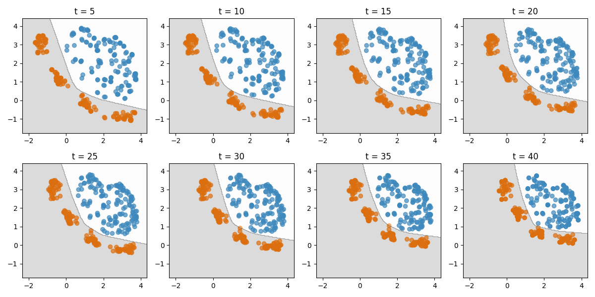
Inspect intermediate states

We can plot the intermediate datasets and decision boundaries.

intermediate_data = gradual_adapter.intermediate_data_

fig, axes = plt.subplots(2, 4, figsize=(12, 6))
axes = axes.ravel()

# Define which steps to plot
steps_to_plot = [5, 10, 15, 20, 25, 30, 35, 40]

for i, step in enumerate(steps_to_plot):
    ax = axes[i]
    X_step, y_step = intermediate_data[step - 1]
    clf = clfs[step - 1]

    ax.scatter(X_step[:, 0], X_step[:, 1], c=y_step, vmax=9, cmap="tab10", alpha=0.7)
    DecisionBoundaryDisplay.from_estimator(
        clf,
        X,
        response_method="predict",
        cmap="gray_r",
        alpha=0.15,
        ax=ax,
        grid_resolution=200,
    )
    ax.set_title(f"t = {step}")
    ax.axis(lims)

plt.tight_layout()

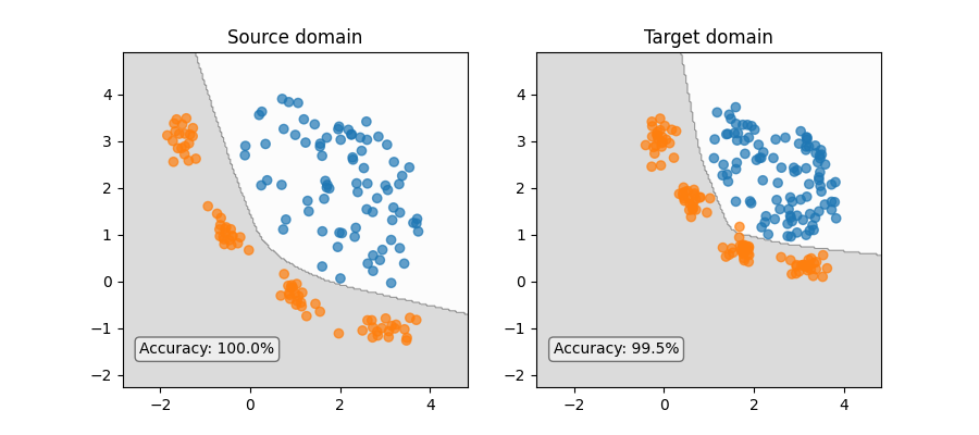
Plot decision boundaries on source and target datasets

Now we can see how this gradual domain adaptation has changed the decision boundary between the source and target domains.

figure, axis = plt.subplots(1, 2, figsize=(9, 4))
cm = "gray_r"
DecisionBoundaryDisplay.from_estimator(
    clfs[0],
    X,
    response_method="predict",
    cmap=cm,
    alpha=0.15,
    ax=axis[0],
    grid_resolution=200,
)
axis[0].scatter(
    X_source[:, 0],
    X_source[:, 1],
    c=y_source,
    vmax=9,
    cmap="tab10",
    alpha=0.7,
)
axis[0].set_title("Source domain")
DecisionBoundaryDisplay.from_estimator(
    clfs[-1],
    X,
    response_method="predict",
    cmap=cm,
    alpha=0.15,
    ax=axis[1],
    grid_resolution=200,
)
axis[1].scatter(
    X_target[:, 0],
    X_target[:, 1],
    c=y_target,
    vmax=9,
    cmap="tab10",
    alpha=0.7,
)
axis[1].set_title("Target domain")

axis[0].text(
    0.05,
    0.1,
    f"Accuracy: {clfs[0].score(X_source, y_source):.1%}",
    transform=axis[0].transAxes,
    ha="left",
    bbox={"boxstyle": "round", "facecolor": "white", "alpha": 0.5},
)
axis[1].text(
    0.05,
    0.1,
    f"Accuracy: {gradual_adapter.score(X_target, y_target):.1%}",
    transform=axis[1].transAxes,
    ha="left",
    bbox={"boxstyle": "round", "facecolor": "white", "alpha": 0.5},
)

plt.show()