DASVM classifier example

This example illustrates the DASVM method from [21].

# Author: Ruben Bueno
#
# License: BSD 3-Clause
# sphinx_gallery_thumbnail_number = 2

import matplotlib.lines as mlines
import matplotlib.pyplot as plt
import numpy as np
from sklearn.base import clone
from sklearn.svm import SVC

from skada import source_target_split
from skada._self_labeling import DASVMClassifier
from skada.datasets import make_dataset_from_moons_distribution

RANDOM_SEED = 42

# base_estimator can be any classifier equipped with `decision_function` such as:
# SVC(kernel='poly'), SVC(kernel='linear'), LogisticRegression(random_state=0), etc...
# however the estimator has been created only for SVC.
base_estimator = SVC()

target_marker = "s"
source_marker = "o"
xlim = (-1.5, 2.4)
ylim = (-1, 1.3)

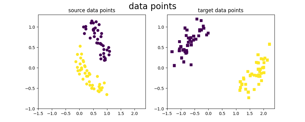
We generate our 2D dataset with 2 classes

We generate a simple 2D dataset from a moon distribution, where source and target are not taken from the same location in the moons. This dataset thus presents a covariate shift.

X, y, sample_domain = make_dataset_from_moons_distribution(
    pos_source=[0.1, 0.2, 0.3, 0.4],
    pos_target=[0.6, 0.7, 0.8, 0.9],
    n_samples_source=10,
    n_samples_target=10,
    noise=0.1,
    random_state=RANDOM_SEED,
)

Xs, Xt, ys, yt = source_target_split(X, y, sample_domain=sample_domain)

Plots of the dataset

As we can see, the source and target datasets have different distributions for the points' positions but have the same labels for the same x-values. We are then in the case of covariate shift.

figure, axis = plt.subplots(1, 2, figsize=(10, 4))

axis[0].scatter(Xs[:, 0], Xs[:, 1], c=ys, marker=source_marker)
axis[0].set_xlim(xlim)
axis[0].set_ylim(ylim)
axis[0].set_title("source data points")

axis[1].scatter(Xt[:, 0], Xt[:, 1], c=yt, marker=target_marker)
axis[1].set_xlim(xlim)
axis[1].set_ylim(ylim)
axis[1].set_title("target data points")

figure.suptitle("data points", fontsize=20)

Text(0.5, 0.98, 'data points')

Usage of the DASVMClassifier

The main problem here is that we only know the distribution of the points from the target dataset, our goal is to label it.

The DASVM method consist in fitting multiple base_estimator (SVC) by:

• Removing from the training dataset (if possible) k points from the source dataset for which the current estimator is doing well

• Adding to the training dataset (if possible) k points from the target dataset for which out current estimator is not so sure about it's prediction (those are target points in the margin band, that are close to the margin)

• Semi-labeling points that were added to the training set and came from the target dataset

• Fit a new estimator on this training set

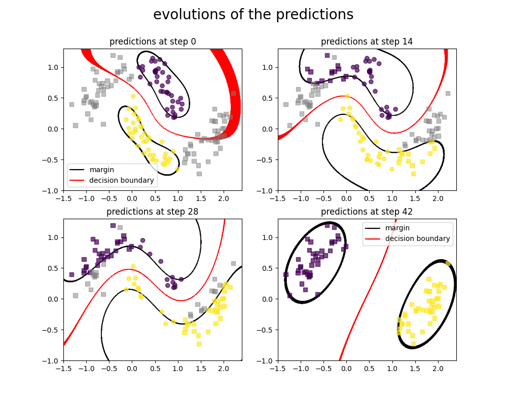
Here we plot the progression of the SVC classifier when training with the DASVM algorithm.

estimator = DASVMClassifier(
    base_estimator=clone(base_estimator), k=5, save_estimators=True, save_indices=True
).fit(X, y, sample_domain=sample_domain)

epsilon = 0.01
K = len(estimator.estimators) // 3
figure, axis = plt.subplots(2, 2, figsize=(2 * 5, 2 * 4))
axis = np.concatenate((axis[0], axis[1]))
for i in list(range(0, len(estimator.estimators), K)) + [-1]:
    j = i // K if i != -1 else -1
    e = estimator.estimators[i]
    x_points = np.linspace(xlim[0], xlim[1], 500)
    y_points = np.linspace(ylim[0], ylim[1], 500)
    X = np.array([[x, y] for x in x_points for y in y_points])

    # plot margins
    if j == -1:
        X_ = X[np.absolute(e.decision_function(X) - 1) < epsilon]
        axis[j].scatter(
            X_[:, 0],
            X_[:, 1],
            c=[1] * X_.shape[0],
            alpha=1,
            cmap="gray",
            s=[0.1] * X_.shape[0],
            label="margin",
        )
        X_ = X[np.absolute(e.decision_function(X) + 1) < epsilon]
        axis[j].scatter(
            X_[:, 0],
            X_[:, 1],
            c=[1] * X_.shape[0],
            alpha=1,
            cmap="gray",
            s=[0.1] * X_.shape[0],
        )
        X_ = X[np.absolute(e.decision_function(X)) < epsilon]
        axis[j].scatter(
            X_[:, 0],
            X_[:, 1],
            c=[1] * X_.shape[0],
            alpha=1,
            cmap="autumn",
            s=[0.1] * X_.shape[0],
            label="decision boundary",
        )
    else:
        X_ = X[np.absolute(e.decision_function(X) - 1) < epsilon]
        axis[j].scatter(
            X_[:, 0],
            X_[:, 1],
            c=[1] * X_.shape[0],
            alpha=1,
            cmap="gray",
            s=[0.1] * X_.shape[0],
        )
        X_ = X[np.absolute(e.decision_function(X) + 1) < epsilon]
        axis[j].scatter(
            X_[:, 0],
            X_[:, 1],
            c=[1] * X_.shape[0],
            alpha=1,
            cmap="gray",
            s=[0.1] * X_.shape[0],
        )
        X_ = X[np.absolute(e.decision_function(X)) < epsilon]
        axis[j].scatter(
            X_[:, 0],
            X_[:, 1],
            c=[1] * X_.shape[0],
            alpha=1,
            cmap="autumn",
            s=[0.1] * X_.shape[0],
        )

    X_s = Xs[~estimator.indices_source_deleted[i]]
    X_t = Xt[estimator.indices_target_added[i]]
    X = np.concatenate((X_s, X_t))

    if sum(estimator.indices_target_added[i]) > 0:
        semi_labels = e.predict(Xt[estimator.indices_target_added[i]])
        axis[j].scatter(
            X_s[:, 0],
            X_s[:, 1],
            c=ys[~estimator.indices_source_deleted[i]],
            marker=source_marker,
            alpha=0.7,
        )
        axis[j].scatter(
            X_t[:, 0], X_t[:, 1], c=semi_labels, marker=target_marker, alpha=0.7
        )
    else:
        semi_labels = np.array([])
        axis[j].scatter(
            X[:, 0], X[:, 1], c=ys[~estimator.indices_source_deleted[i]], alpha=0.7
        )
    X = Xt[~estimator.indices_target_added[i]]
    axis[j].scatter(
        X[:, 0],
        X[:, 1],
        cmap="gray",
        c=[0.5] * X.shape[0],
        alpha=0.5,
        vmax=1,
        vmin=0,
        marker=target_marker,
    )

    axis[j].set_xlim(xlim)
    axis[j].set_ylim(ylim)
    if i == -1:
        i = len(estimator.estimators)
    axis[j].set_title(f"predictions at step {i}")

figure.suptitle("evolutions of the predictions", fontsize=20)

margin_line = mlines.Line2D(
    [], [], color="black", marker="_", markersize=15, label="margin"
)
decision_boundary = mlines.Line2D(
    [], [], color="red", marker="_", markersize=15, label="decision boundary"
)
axis[0].legend(handles=[margin_line, decision_boundary], loc="lower left")
axis[-1].legend(handles=[margin_line, decision_boundary])

<matplotlib.legend.Legend object at 0x7f53e241e5c0>

Labeling the target dataset

Here we show 4 states from our algorithm, At first we are only given source data points with label (which are circle, in colors showing the label), and target datapoints that have no labels (which are represented as squares, in gray when they have no labels)

As we go further in the algorithm steps, we can notice that more and more of the target datapoints (squares) are now labeled, while more and more of the source datapoints (circles) are removed from the training set.

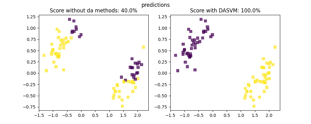
# We show the improvement of the labeling technique.
figure, axis = plt.subplots(1, 2, figsize=(10, 4))
semi_labels = (base_estimator.fit(Xs, ys).predict(Xt), estimator.predict(Xt))
axis[0].scatter(Xt[:, 0], Xt[:, 1], c=semi_labels[0], alpha=0.7, marker=target_marker)
axis[1].scatter(Xt[:, 0], Xt[:, 1], c=semi_labels[1], alpha=0.7, marker=target_marker)

scores = (
    np.array([sum(semi_labels[0] == yt), sum(semi_labels[1] == yt)])
    * 100
    / semi_labels[0].shape[0]
)

axis[0].set_title(f"Score without da methods: {scores[0]}%")
axis[1].set_title(f"Score with DASVM: {scores[1]}%")
figure.suptitle("predictions")
plt.show()