Note
Go to the end to download the full example code.
Optimal Transport Domain Adaptation (OTDA)
This example illustrates the OTDA method from [1] on a simple classification task.
# Author: Remi Flamary
#
# License: BSD 3-Clause
# sphinx_gallery_thumbnail_number = 4
import matplotlib.pyplot as plt
from sklearn.inspection import DecisionBoundaryDisplay
from sklearn.svm import SVC

from skada import (
    ClassRegularizerOTMappingAdapter,
    EntropicOTMappingAdapter,
    LinearOTMappingAdapter,
    OTMapping,
    make_da_pipeline,
    source_target_split,
)
from skada.datasets import make_shifted_datasets
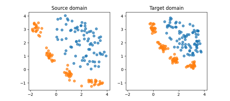
Generate conditional shift dataset
n_samples = 20
X, y, sample_domain = make_shifted_datasets(
    n_samples_source=n_samples,
    n_samples_target=n_samples + 1,
    shift="conditional_shift",
    noise=0.1,
    random_state=42,
)


X_source, X_target, y_source, y_target = source_target_split(
    X, y, sample_domain=sample_domain
)


n_tot_source = X_source.shape[0]
n_tot_target = X_target.shape[0]

plt.figure(1, figsize=(8, 3.5))
plt.subplot(121)

plt.scatter(X_source[:, 0], X_source[:, 1], c=y_source, vmax=9, cmap="tab10", alpha=0.7)
plt.title("Source domain")
lims = plt.axis()

plt.subplot(122)
plt.scatter(X_target[:, 0], X_target[:, 1], c=y_target, vmax=9, cmap="tab10", alpha=0.7)
plt.title("Target domain")
plt.axis(lims)
(np.float64(-2.1321138905671275), np.float64(4.218866137683906), np.float64(-1.5244703189443227), np.float64(4.288146109474553))
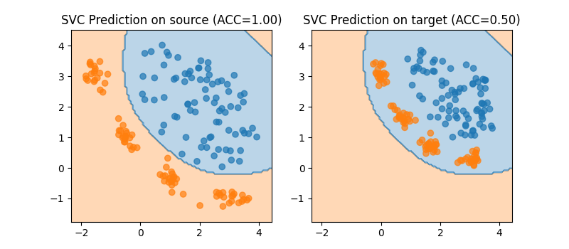
Illustration of the DA problem
# Train on source

clf = SVC(kernel="rbf", C=1)
clf.fit(X_source, y_source)

# Compute accuracy on source and target
ACC_source = clf.score(X_source, y_source)
ACC_target = clf.score(X_target, y_target)

plt.figure(2, figsize=(8, 3.5))
plt.subplot(121)
DecisionBoundaryDisplay.from_estimator(
    clf,
    X_source,
    alpha=0.3,
    eps=0.5,
    response_method="predict",
    vmax=9,
    cmap="tab10",
    ax=plt.gca(),
)
plt.scatter(X_source[:, 0], X_source[:, 1], c=y_source, vmax=9, cmap="tab10", alpha=0.7)
plt.title(f"SVC Prediction on source (ACC={ACC_source:.2f})")
lims = plt.axis()

plt.subplot(122)
DecisionBoundaryDisplay.from_estimator(
    clf,
    X_source,
    alpha=0.3,
    eps=0.5,
    response_method="predict",
    vmax=9,
    cmap="tab10",
    ax=plt.gca(),
)
plt.scatter(X_target[:, 0], X_target[:, 1], c=y_target, vmax=9, cmap="tab10", alpha=0.7)
plt.title(f"SVC Prediction on target (ACC={ACC_target:.2f})")
lims = plt.axis()
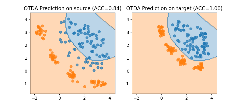
Optimal Transport Domain Adaptation
clf_otda = OTMapping(SVC(kernel="rbf", C=1))
clf_otda.fit(X, y, sample_domain=sample_domain)

# Compute accuracy on source and target
ACC_source = clf_otda.score(X_source, y_source)
ACC_target = clf_otda.score(X_target, y_target)

plt.figure(3, figsize=(8, 3.5))
plt.subplot(121)
DecisionBoundaryDisplay.from_estimator(
    clf_otda,
    X_source,
    alpha=0.3,
    eps=0.5,
    response_method="predict",
    vmax=9,
    cmap="tab10",
    ax=plt.gca(),
)
plt.scatter(X_source[:, 0], X_source[:, 1], c=y_source, vmax=9, cmap="tab10", alpha=0.7)
plt.title(f"OTDA Prediction on source (ACC={ACC_source:.2f})")
lims = plt.axis()

plt.subplot(122)
DecisionBoundaryDisplay.from_estimator(
    clf_otda,
    X_source,
    alpha=0.3,
    eps=0.5,
    response_method="predict",
    vmax=9,
    cmap="tab10",
    ax=plt.gca(),
)
plt.scatter(X_target[:, 0], X_target[:, 1], c=y_target, vmax=9, cmap="tab10", alpha=0.7)
plt.title(f"OTDA Prediction on target (ACC={ACC_target:.2f})")
lims = plt.axis()
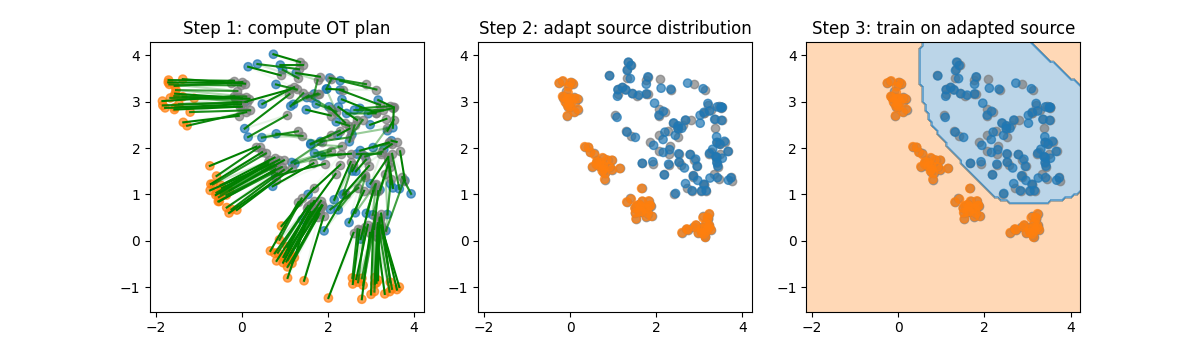
How does OTDA works?
The OTDA method is based on the following idea: the optimal transport between the source and target feature distribution is computed (which gives us what is called an optimal plan). Then, the source samples are mapped to the target distribution using this optimal plan and the classifier is trained on the mapped # samples.
We illustrate below the different steps of the OTDA method.
# recovering the OT plan
adapter = clf_otda.named_steps["otmappingadapter"].get_estimator()
T = adapter.ot_transport_.coupling_
T = T / T.max()

# computing the transported samples
X_adapted = clf_otda[:-1].transform(X, sample_domain=sample_domain, allow_source=True)
# this could also be done with 'select_domain' helper
X_source_adapted = X_adapted[sample_domain > 0]

plt.figure(4, figsize=(12, 3.5))
plt.subplot(131)
for i in range(n_tot_source):
    for j in range(n_tot_target):
        if T[i, j] > 0:
            plt.plot(
                [X_source[i, 0], X_target[j, 0]],
                [X_source[i, 1], X_target[j, 1]],
                "-g",
                alpha=T[i, j],
            )
plt.scatter(X_source[:, 0], X_source[:, 1], c=y_source, vmax=9, cmap="tab10", alpha=0.7)
plt.scatter(X_target[:, 0], X_target[:, 1], c="C7", alpha=0.7)
plt.title(label="Step 1: compute OT plan")
lims = plt.axis()

plt.subplot(132)
plt.scatter(X_target[:, 0], X_target[:, 1], c="C7", alpha=0.7)
plt.scatter(
    X_source_adapted[:, 0],
    X_source_adapted[:, 1],
    c=y_source,
    vmax=9,
    cmap="tab10",
    alpha=0.7,
)
plt.axis(lims)
plt.title(label="Step 2: adapt source distribution")

plt.subplot(133)
DecisionBoundaryDisplay.from_estimator(
    clf_otda,
    X_source,
    alpha=0.3,
    eps=0.5,
    response_method="predict",
    vmax=9,
    cmap="tab10",
    ax=plt.gca(),
)
plt.scatter(X_target[:, 0], X_target[:, 1], c="C7", alpha=0.7)
plt.scatter(
    X_source_adapted[:, 0],
    X_source_adapted[:, 1],
    c=y_source,
    vmax=9,
    cmap="tab10",
    alpha=0.7,
)
plt.axis(lims)
plt.title(label="Step 3: train on adapted source")
Text(0.5, 1.0, 'Step 3: train on adapted source')
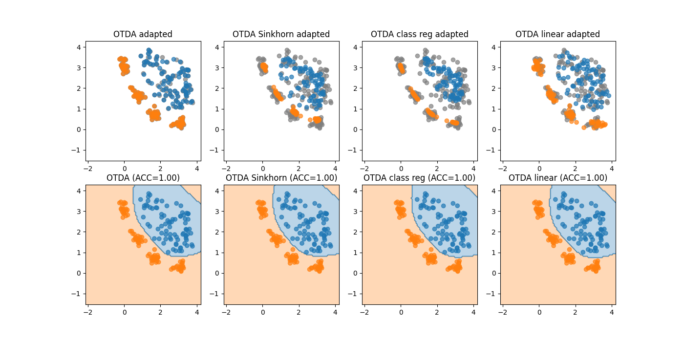
Different OTDA methods
The OTDA method can be used with different optimal transport solvers. Here we illustrate the different methods available in SKADA.
# Sinkhorn OT solver
clf_otda_sinkhorn = make_da_pipeline(
    EntropicOTMappingAdapter(reg_e=1), SVC(kernel="rbf", C=1)
)
clf_otda_sinkhorn.fit(X, y, sample_domain=sample_domain)
ACC_sinkhorn = clf_otda_sinkhorn.score(
    X,
    y,
    sample_domain=sample_domain,
    allow_source=True,
)
X_adapted_sinkhorn = clf_otda_sinkhorn[:-1].transform(
    X,
    sample_domain=sample_domain,
    allow_source=True,
)
X_source_adapted_sinkhorn = X_adapted_sinkhorn[sample_domain > 0]

# Sinkhorn OT solver with class regularization
clf_otds_classreg = make_da_pipeline(
    ClassRegularizerOTMappingAdapter(reg_e=1.0, reg_cl=1.0), SVC(kernel="rbf", C=1)
)
clf_otds_classreg.fit(X, y, sample_domain=sample_domain)
ACC_classreg = clf_otds_classreg.score(
    X,
    y,
    sample_domain=sample_domain,
    allow_source=True,
)
X_adapted_classreg = clf_otds_classreg[:-1].transform(
    X,
    sample_domain=sample_domain,
    allow_source=True,
)
X_source_adapted_classreg = X_adapted_classreg[sample_domain > 0]

# Linear OT solver
clf_otda_linear = make_da_pipeline(LinearOTMappingAdapter(), SVC(kernel="rbf", C=1))
clf_otda_linear.fit(X, y, sample_domain=sample_domain)
ACC_linear = clf_otda_linear.score(
    X,
    y,
    sample_domain=sample_domain,
    allow_source=True,
)
X_adapted_linear = clf_otda_linear[:-1].transform(
    X,
    sample_domain=sample_domain,
    allow_source=True,
)
X_source_adapted_linear = X_adapted_linear[sample_domain > 0]

plt.figure(5, figsize=(14, 7))

plt.subplot(241)
plt.scatter(X_target[:, 0], X_target[:, 1], c="C7", alpha=0.7)
plt.scatter(
    X_source_adapted[:, 0],
    X_source_adapted[:, 1],
    c=y_source,
    vmax=9,
    cmap="tab10",
    alpha=0.7,
)
plt.axis(lims)
plt.title(label="OTDA adapted")

plt.subplot(242)
plt.scatter(X_target[:, 0], X_target[:, 1], c="C7", alpha=0.7)
plt.scatter(
    X_source_adapted_sinkhorn[:, 0],
    X_source_adapted_sinkhorn[:, 1],
    c=y_source,
    vmax=9,
    cmap="tab10",
    alpha=0.7,
)
plt.axis(lims)
plt.title(label="OTDA Sinkhorn adapted")

plt.subplot(243)
plt.scatter(X_target[:, 0], X_target[:, 1], c="C7", alpha=0.7)
plt.scatter(
    X_source_adapted_classreg[:, 0],
    X_source_adapted_classreg[:, 1],
    c=y_source,
    vmax=9,
    cmap="tab10",
    alpha=0.7,
)
plt.axis(lims)
plt.title(label="OTDA class reg adapted")

plt.subplot(244)
plt.scatter(X_target[:, 0], X_target[:, 1], c="C7", alpha=0.7)
plt.scatter(
    X_source_adapted_linear[:, 0],
    X_source_adapted_linear[:, 1],
    c=y_source,
    vmax=9,
    cmap="tab10",
    alpha=0.7,
)
plt.axis(lims)
plt.title(label="OTDA linear adapted")

plt.subplot(245)
DecisionBoundaryDisplay.from_estimator(
    clf_otda,
    X_source,
    alpha=0.3,
    eps=0.5,
    response_method="predict",
    vmax=9,
    cmap="tab10",
    ax=plt.gca(),
)
plt.scatter(X_target[:, 0], X_target[:, 1], c=y_target, vmax=9, cmap="tab10", alpha=0.7)
plt.axis(lims)
plt.title(label=f"OTDA (ACC={ACC_target:.2f})")

plt.subplot(246)
DecisionBoundaryDisplay.from_estimator(
    clf_otda_sinkhorn,
    X_source,
    alpha=0.3,
    eps=0.5,
    response_method="predict",
    vmax=9,
    cmap="tab10",
    ax=plt.gca(),
)
plt.scatter(X_target[:, 0], X_target[:, 1], c=y_target, vmax=9, cmap="tab10", alpha=0.7)
plt.axis(lims)
plt.title(label=f"OTDA Sinkhorn (ACC={ACC_sinkhorn:.2f})")

plt.subplot(247)
DecisionBoundaryDisplay.from_estimator(
    clf_otds_classreg,
    X_source,
    alpha=0.3,
    eps=0.5,
    response_method="predict",
    vmax=9,
    cmap="tab10",
    ax=plt.gca(),
)
plt.scatter(X_target[:, 0], X_target[:, 1], c=y_target, vmax=9, cmap="tab10", alpha=0.7)
plt.axis(lims)
plt.title(label=f"OTDA class reg (ACC={ACC_classreg:.2f})")

plt.subplot(248)
DecisionBoundaryDisplay.from_estimator(
    clf_otda_linear,
    X_source,
    alpha=0.3,
    eps=0.5,
    response_method="predict",
    vmax=9,
    cmap="tab10",
    ax=plt.gca(),
)
plt.scatter(X_target[:, 0], X_target[:, 1], c=y_target, vmax=9, cmap="tab10", alpha=0.7)
plt.axis(lims)
plt.title(label=f"OTDA linear (ACC={ACC_linear:.2f})")
/home/circleci/.local/lib/python3.10/site-packages/ot/bregman/_sinkhorn.py:666: UserWarning: Sinkhorn did not converge. You might want to increase the number of iterations `numItermax` or the regularization parameter `reg`.
  warnings.warn(

Text(0.5, 1.0, 'OTDA linear (ACC=1.00)')
Total running time of the script: (0 minutes 1.786 seconds)