JDOT Regressor and Classifier examples

This example shows how to use the JDOTRegressor [10] to learn a regression model from source to target domain on a simple concept drift 2D example. We use a simple Kernel Ridge Regression (KRR) as base estimator.

We compare the performance of the KRR on the source and target domain, and the JDOTRegressor on the same task and illustrate the learned decision boundary and the OT plan between samples estimated by JDOT.

[10]

Courty, N., Flamary, R., Habrard, A., & Rakotomamonjy, A. (2017). Joint distribution optimal transportation for domain adaptation. Advances in neural information processing systems, 30.

# Author: Remi Flamary
#
# License: BSD 3-Clause
# sphinx_gallery_thumbnail_number = 4

import matplotlib.pyplot as plt
import numpy as np
from sklearn.kernel_ridge import KernelRidge
from sklearn.linear_model import LogisticRegression
from sklearn.metrics import mean_squared_error
from sklearn.svm import SVC

from skada import JDOTClassifier, JDOTRegressor, source_target_split
from skada.datasets import make_shifted_datasets

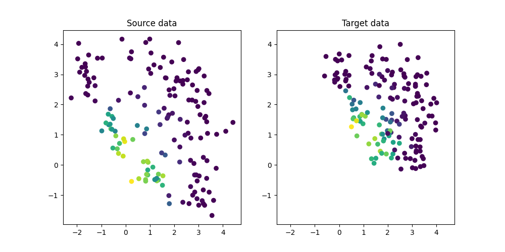
Generate concept drift regression dataset and plot it

We generate a simple 2D concept drift dataset.

X, y, sample_domain = make_shifted_datasets(
    n_samples_source=20,
    n_samples_target=20,
    shift="concept_drift",
    noise=0.3,
    label="regression",
    random_state=42,
)

y = (y - y.mean()) / y.std()

Xs, Xt, ys, yt = source_target_split(X, y, sample_domain=sample_domain)


plt.figure(1, (10, 5))
plt.subplot(1, 2, 1)
plt.scatter(Xs[:, 0], Xs[:, 1], c=ys, label="Source")
plt.title("Source data")
ax = plt.axis()

plt.subplot(1, 2, 2)
plt.scatter(Xt[:, 0], Xt[:, 1], c=yt, label="Target")
plt.title("Target data")
plt.axis(ax)

(np.float64(-2.570318895725525), np.float64(4.744989537549497), np.float64(-1.9610814126500358), np.float64(4.45933195939893))

Train a regressor on source data

We train a simple Kernel Ridge Regression (KRR) on the source domain and evaluate its performance on the source and target domain. Performance is much lower on the target domain due to the shift. We also plot the decision boundary learned by the KRR.

clf = KernelRidge(kernel="rbf", alpha=0.5)
clf.fit(Xs, ys)

# Compute accuracy on source and target
ys_pred = clf.predict(Xs)
yt_pred = clf.predict(Xt)

mse_s = mean_squared_error(ys, ys_pred)
mse_t = mean_squared_error(yt, yt_pred)

print(f"MSE on source: {mse_s:.2f}")
print(f"MSE on target: {mse_t:.2f}")

XX, YY = np.meshgrid(np.linspace(ax[0], ax[1], 100), np.linspace(ax[2], ax[3], 100))
Z = clf.predict(np.c_[XX.ravel(), YY.ravel()]).reshape(XX.shape)


plt.figure(2, (10, 5))
plt.subplot(1, 2, 1)
plt.scatter(Xs[:, 0], Xs[:, 1], c=ys, label="Prediction")
plt.imshow(Z, extent=(ax[0], ax[1], ax[2], ax[3]), origin="lower", alpha=0.5)
plt.title(f"KRR Prediction on source (MSE={mse_s:.2f})")
plt.axis(ax)

plt.subplot(1, 2, 2)
plt.scatter(Xt[:, 0], Xt[:, 1], c=yt, label="Prediction")
plt.imshow(Z, extent=(ax[0], ax[1], ax[2], ax[3]), origin="lower", alpha=0.5)
plt.title(f"KRR Prediction on target (MSE={mse_t:.2f})")
plt.axis(ax)

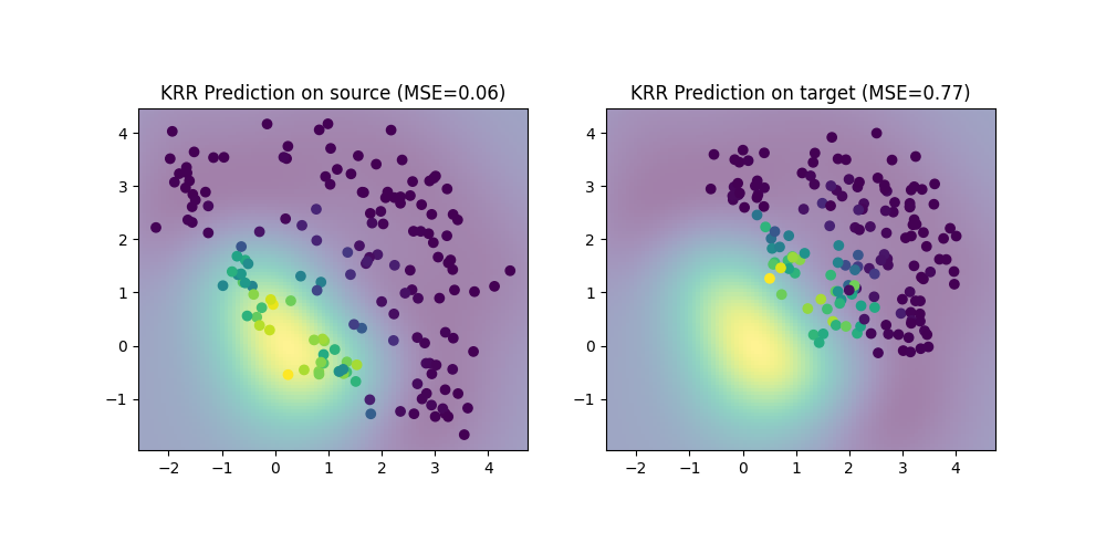
MSE on source: 0.06
MSE on target: 0.77

(np.float64(-2.570318895725525), np.float64(4.744989537549497), np.float64(-1.9610814126500358), np.float64(4.45933195939893))

Train with JDOT regressor

We now use the JDOTRegressor to learn a regression model from source to target domain. We use the same KRR as base estimator. We compare the performance of JDOT on the source and target domain, and illustrate the learned decision boundary of JDOT. Performance is much better on the target domain than with the KRR trained on source.

jdot = JDOTRegressor(base_estimator=KernelRidge(kernel="rbf", alpha=0.5), alpha=0.01)

jdot.fit(X, y, sample_domain=sample_domain)

ys_pred = jdot.predict(Xs)
yt_pred = jdot.predict(Xt)

mse_s = mean_squared_error(ys, ys_pred)
mse_t = mean_squared_error(yt, yt_pred)

Zjdot = jdot.predict(np.c_[XX.ravel(), YY.ravel()]).reshape(XX.shape)

print(f"JDOT MSE on source: {mse_s:.2f}")
print(f"JDOT MSE on target: {mse_t:.2f}")

plt.figure(3, (10, 5))
plt.subplot(1, 2, 1)
plt.scatter(Xs[:, 0], Xs[:, 1], c=ys, label="Prediction")
plt.imshow(Zjdot, extent=(ax[0], ax[1], ax[2], ax[3]), origin="lower", alpha=0.5)
plt.title(f"JDOT Prediction on source (MSE={mse_s:.2f})")
plt.axis(ax)

plt.subplot(1, 2, 2)
plt.scatter(Xt[:, 0], Xt[:, 1], c=yt, label="Prediction")
plt.imshow(Zjdot, extent=(ax[0], ax[1], ax[2], ax[3]), origin="lower", alpha=0.5)
plt.title(f"JDOT Prediction on target (MSE={mse_t:.2f})")
plt.axis(ax)

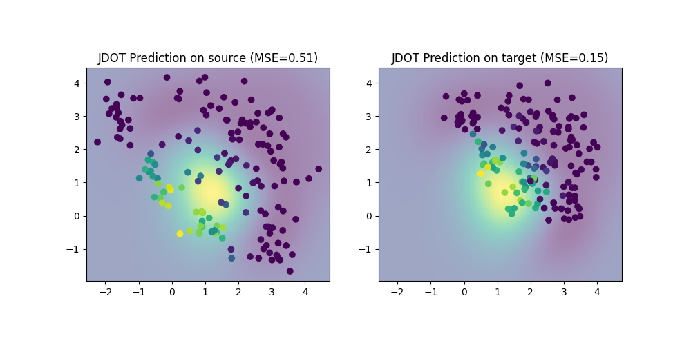
JDOT MSE on source: 0.51
JDOT MSE on target: 0.15

(np.float64(-2.570318895725525), np.float64(4.744989537549497), np.float64(-1.9610814126500358), np.float64(4.45933195939893))

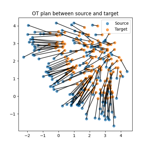
Illustration of the OT plan

We illustrate the OT plan between samples estimated by JDOT. We plot the OT plan between the source and target samples. We can see that the OT plan is able to align the source and target samples while preserving the label.

T = jdot.sol_.plan
T = T / T.max()

plt.figure(4, (5, 5))

plt.scatter(Xs[:, 0], Xs[:, 1], c="C0", label="Source", alpha=0.7)
plt.scatter(Xt[:, 0], Xt[:, 1], c="C1", label="Target", alpha=0.7)

for i in range(Xs.shape[0]):
    for j in range(Xt.shape[0]):
        if T[i, j] > 0.01:
            plt.plot(
                [Xs[i, 0], Xt[j, 0]], [Xs[i, 1], Xt[j, 1]], "k", alpha=T[i, j] * 0.8
            )
plt.legend()
plt.title("OT plan between source and target")

Text(0.5, 1.0, 'OT plan between source and target')

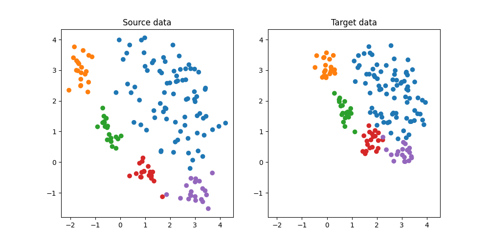
Generate concept drift classification dataset and plot it

We generate a simple 2D concept drift dataset.

X, y, sample_domain = make_shifted_datasets(
    n_samples_source=20,
    n_samples_target=20,
    shift="concept_drift",
    noise=0.2,
    label="multiclass",
    random_state=42,
)


Xs, Xt, ys, yt = source_target_split(X, y, sample_domain=sample_domain)


plt.figure(5, (10, 5))
plt.subplot(1, 2, 1)
plt.scatter(Xs[:, 0], Xs[:, 1], c=ys, cmap="tab10", vmax=9, label="Source")
plt.title("Source data")
ax = plt.axis()

plt.subplot(1, 2, 2)
plt.scatter(Xt[:, 0], Xt[:, 1], c=yt, cmap="tab10", vmax=9, label="Target")
plt.title("Target data")
plt.axis(ax)

(np.float64(-2.3676169789533272), np.float64(4.53817259426296), np.float64(-1.7964573229829714), np.float64(4.336863129384494))

Train a classifier on source data

We train a simple SVC classifier on the source domain and evaluate its performance on the source and target domain. Performance is much lower on the target domain due to the shift. We also plot the decision boundary

clf = LogisticRegression()
clf.fit(Xs, ys)

# Compute accuracy on source and target
ys_pred = clf.predict(Xs)
yt_pred = clf.predict(Xt)

acc_s = (ys_pred == ys).mean()
acc_t = (yt_pred == yt).mean()

print(f"Accuracy on source: {acc_s:.2f}")
print(f"Accuracy on target: {acc_t:.2f}")

XX, YY = np.meshgrid(np.linspace(ax[0], ax[1], 100), np.linspace(ax[2], ax[3], 100))
Z = clf.predict(np.c_[XX.ravel(), YY.ravel()]).reshape(XX.shape)


plt.figure(6, (10, 5))
plt.subplot(1, 2, 1)
plt.scatter(Xs[:, 0], Xs[:, 1], c=ys, cmap="tab10", vmax=9, label="Prediction")
plt.imshow(
    Z,
    extent=(ax[0], ax[1], ax[2], ax[3]),
    origin="lower",
    alpha=0.5,
    cmap="tab10",
    vmax=9,
)
plt.title(f"SVC Prediction on source (ACC={acc_s:.2f})")

plt.subplot(1, 2, 2)
plt.scatter(Xt[:, 0], Xt[:, 1], c=yt, cmap="tab10", vmax=9, label="Prediction")
plt.imshow(
    Z,
    extent=(ax[0], ax[1], ax[2], ax[3]),
    origin="lower",
    alpha=0.5,
    cmap="tab10",
    vmax=9,
)
plt.title(f"SVC Prediction on target (ACC={acc_t:.2f})")
plt.axis(ax)

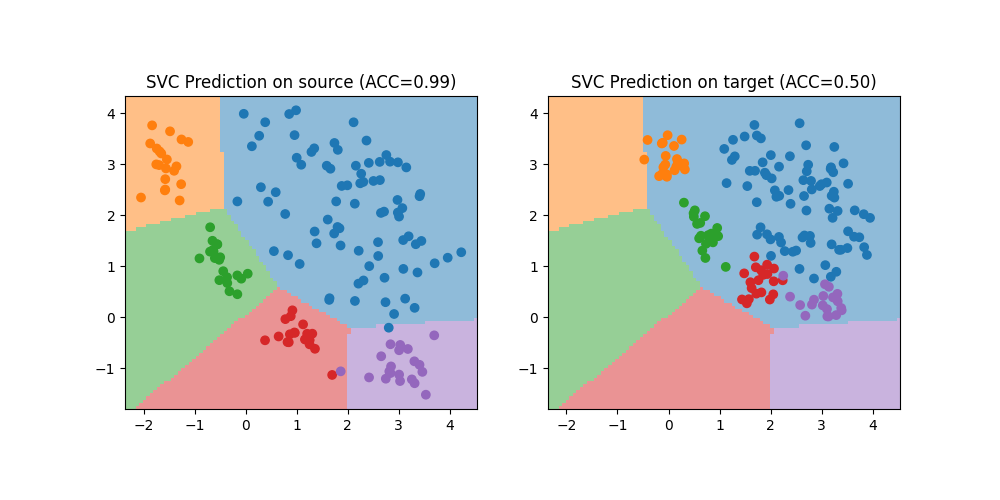
Accuracy on source: 0.99
Accuracy on target: 0.50

(np.float64(-2.3676169789533272), np.float64(4.53817259426296), np.float64(-1.7964573229829714), np.float64(4.336863129384494))

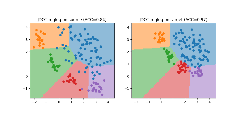
Train with JDOT classifier

We now use the JDOTClassifier to learn a classification model from source to target domain. We use the same SVC as base estimator. We compare the performance of JDOT on the source and target domain, and illustrate the learned decision boundary of JDOT. Performance is much better on the target domain than with the SVC trained on source.

jdot = JDOTClassifier(LogisticRegression(), verbose=True)

jdot.fit(X, y, sample_domain=sample_domain)

ys_pred = jdot.predict(Xs)
yt_pred = jdot.predict(Xt)

acc_s = (ys_pred == ys).mean()
acc_t = (yt_pred == yt).mean()

print(f"JDOT Accuracy on source: {acc_s:.2f}")
print(f"JDOT Accuracy on target: {acc_t:.2f}")

XX, YY = np.meshgrid(np.linspace(ax[0], ax[1], 100), np.linspace(ax[2], ax[3], 100))
Z = jdot.predict(np.c_[XX.ravel(), YY.ravel()]).reshape(XX.shape)


plt.figure(7, (10, 5))
plt.subplot(1, 2, 1)
plt.scatter(Xs[:, 0], Xs[:, 1], c=ys, cmap="tab10", vmax=9, label="Prediction")
plt.imshow(
    Z,
    extent=(ax[0], ax[1], ax[2], ax[3]),
    origin="lower",
    alpha=0.5,
    cmap="tab10",
    vmax=9,
)
plt.title(f"JDOT reglog on source (ACC={acc_s:.2f})")

plt.subplot(1, 2, 2)
plt.scatter(Xt[:, 0], Xt[:, 1], c=yt, cmap="tab10", vmax=9, label="Prediction")
plt.imshow(
    Z,
    extent=(ax[0], ax[1], ax[2], ax[3]),
    origin="lower",
    alpha=0.5,
    cmap="tab10",
    vmax=9,
)
plt.title(f"JDOT reglog on target (ACC={acc_t:.2f})")
plt.axis(ax)

iter=0, loss_ot=5.075493682966016, loss_tgt_labels=0.22983129554592746
iter=1, loss_ot=0.18530735809550572, loss_tgt_labels=0.21420445266620786
iter=2, loss_ot=0.18279941870395425, loss_tgt_labels=0.21420445266620786
JDOT Accuracy on source: 0.84
JDOT Accuracy on target: 0.97

(np.float64(-2.3676169789533272), np.float64(4.53817259426296), np.float64(-1.7964573229829714), np.float64(4.336863129384494))

Train with JDOT classifier with SVC

We now use the JDOTClassifier with a support vector classifier as base estimator to learn a classification model from source to target domain. Note that in this case it is necessary to change the metric from the default 'multinomial' to 'hinge' to match the hinge loss used by the SVC.

jdot = JDOTClassifier(SVC(kernel="rbf", C=1), metric="hinge")

jdot.fit(X, y, sample_domain=sample_domain)

ys_pred = jdot.predict(Xs)
yt_pred = jdot.predict(Xt)

acc_s = (ys_pred == ys).mean()
acc_t = (yt_pred == yt).mean()

print(f"JDOT Accuracy on source: {acc_s:.2f}")
print(f"JDOT Accuracy on target: {acc_t:.2f}")

XX, YY = np.meshgrid(np.linspace(ax[0], ax[1], 100), np.linspace(ax[2], ax[3], 100))
Z = jdot.predict(np.c_[XX.ravel(), YY.ravel()]).reshape(XX.shape)


plt.figure(8, (10, 5))
plt.subplot(1, 2, 1)
plt.scatter(Xs[:, 0], Xs[:, 1], c=ys, cmap="tab10", vmax=9, label="Prediction")
plt.imshow(
    Z,
    extent=(ax[0], ax[1], ax[2], ax[3]),
    origin="lower",
    alpha=0.5,
    cmap="tab10",
    vmax=9,
)
plt.title(f"JDOT SVC on source (ACC={acc_s:.2f})")

plt.subplot(1, 2, 2)
plt.scatter(Xt[:, 0], Xt[:, 1], c=yt, cmap="tab10", vmax=9, label="Prediction")
plt.imshow(
    Z,
    extent=(ax[0], ax[1], ax[2], ax[3]),
    origin="lower",
    alpha=0.5,
    cmap="tab10",
    vmax=9,
)
plt.title(f"JDOT SVC on target (ACC={acc_t:.2f})")
plt.axis(ax)

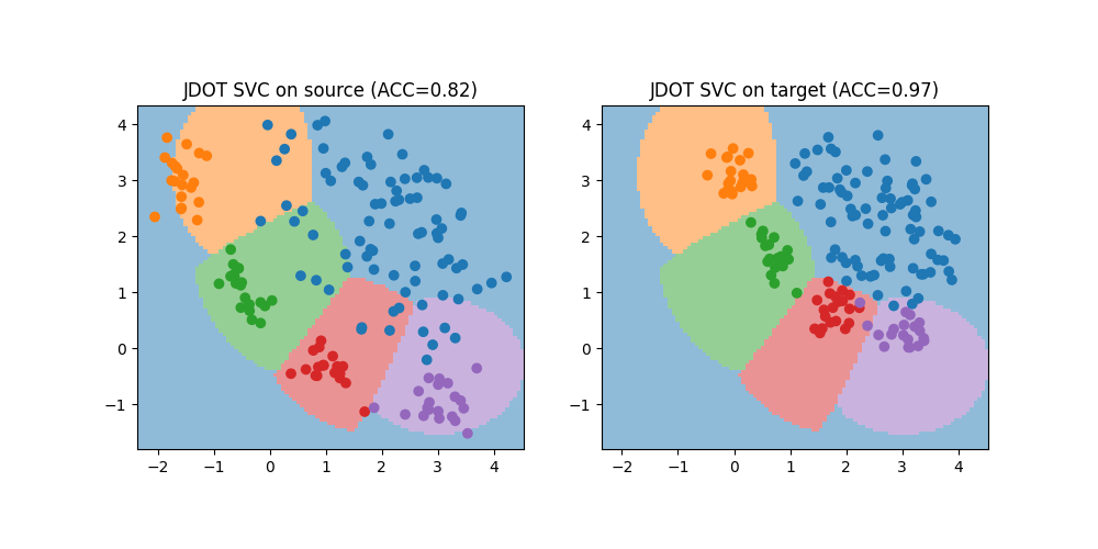
JDOT Accuracy on source: 0.82
JDOT Accuracy on target: 0.97

(np.float64(-2.3676169789533272), np.float64(4.53817259426296), np.float64(-1.7964573229829714), np.float64(4.336863129384494))