Reweighting method example on covariate shift dataset

An example of the reweighting methods on a dataset subject to covariate shift

# Author:   Ruben Bueno <ruben.bueno@polytechnique.edu>
#           Antoine de Mathelin
#           Oleksii Kachaiev <kachayev@gmail.com>
#
# License: BSD 3-Clause
# sphinx_gallery_thumbnail_number = 7

import matplotlib.pyplot as plt
import numpy as np
from matplotlib.colors import ListedColormap
from sklearn.inspection import DecisionBoundaryDisplay
from sklearn.linear_model import LogisticRegression
from sklearn.neighbors import KernelDensity

from skada import (
    DensityReweight,
    DiscriminatorReweight,
    GaussianReweight,
    KLIEPReweight,
    KMMReweight,
    NearestNeighborReweight,
    source_target_split,
)
from skada.datasets import make_shifted_datasets
from skada.utils import extract_source_indices

Reweighting Methods

The purpose of reweighting methods is to estimate weights for the source dataset. These weights are then used to fit an estimator on the source dataset, taking the weights into account. The goal is to ensure that the fitted estimator is suitable for predicting labels from the target distribution.

Reweighting methods implemented and illustrated are the following:

• Density Reweighting

• Gaussian Reweighting

• Discr. Reweighting

• KLIEPReweight

• Nearest Neighbor reweighting

• Kernel Mean Matching

For more details, look at [3].

[3]

[Sugiyama et al., 2008] Sugiyama, M., Suzuki, T., Nakajima, S., Kashima, H., von Bünau, P., and Kawanabe, M. (2008). Direct importance estimation for covariate shift adaptation. Annals of the Institute of Statistical Mathematics, 60(4):699–746. https://www.ism.ac.jp/editsec/aism/pdf/060_4_0699.pdf

base_classifier = LogisticRegression().set_fit_request(sample_weight=True)

print(f"Will be using {base_classifier} as base classifier", end="\n\n")

Will be using LogisticRegression() as base classifier

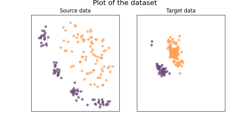
We generate our 2D dataset with 2 classes

We generate a simple 2D dataset with covariate shift

RANDOM_SEED = 42

X, y, sample_domain = make_shifted_datasets(
    n_samples_source=20, n_samples_target=20, noise=0.1, random_state=RANDOM_SEED
)

Xs, Xt, ys, yt = source_target_split(X, y, sample_domain=sample_domain)

Plot of the dataset:

x_min, x_max = -2.5, 4.5
y_min, y_max = -1.5, 4.5


figsize = (8, 4)
figure, axes = plt.subplots(1, 2, figsize=figsize)

cm = plt.cm.RdBu
colormap = ListedColormap(["#FFA056", "#6C4C7C"])
ax = axes[0]
ax.set_title("Source data")
# Plot the source points:
ax.scatter(Xs[:, 0], Xs[:, 1], c=ys, cmap=colormap, alpha=0.7, s=[25])

ax.set_xticks(()), ax.set_yticks(())
ax.set_xlim(x_min, x_max), ax.set_ylim(y_min, y_max)

ax = axes[1]

ax.set_title("Target data")
# Plot the target points:
ax.scatter(Xt[:, 0], Xt[:, 1], c=ys, cmap=colormap, alpha=0.1, s=[25])
ax.scatter(Xt[:, 0], Xt[:, 1], c=yt, cmap=colormap, alpha=0.7, s=[25])
figure.suptitle("Plot of the dataset", fontsize=16, y=1)
ax.set_xticks(()), ax.set_yticks(())
ax.set_xlim(x_min, x_max), ax.set_ylim(y_min, y_max)

((-2.5, 4.5), (-1.5, 4.5))

Illustration of the problem with no domain adaptation

When not using domain adaptation, the classifier won't train on data that is distributed as the target sample domain, it will thus not be performing optimaly.

# We create a dict to store scores:
scores_dict = {}


def plot_weights_and_classifier(
    clf,
    weights,
    name="Without DA",
    suptitle=None,
):
    if suptitle is None:
        suptitle = f"Illustration of the {name} method"
    figure, axes = plt.subplots(1, 2, figsize=figsize)
    ax = axes[1]
    score = clf.score(Xt, yt)
    DecisionBoundaryDisplay.from_estimator(
        clf,
        Xs,
        cmap=ListedColormap(["w", "k"]),
        alpha=1,
        ax=ax,
        eps=0.5,
        response_method="predict",
        plot_method="contour",
    )

    size = 5 + 10 * weights

    # Plot the target points:
    ax.scatter(
        Xt[:, 0],
        Xt[:, 1],
        c=yt,
        cmap=colormap,
        alpha=0.7,
        s=[25],
    )

    ax.set_xticks(()), ax.set_yticks(())
    ax.set_xlim(x_min, x_max), ax.set_ylim(y_min, y_max)
    ax.set_title("Accuracy on target", fontsize=12)
    ax.text(
        x_max - 0.3,
        y_min + 0.3,
        ("%.2f" % score).lstrip("0"),
        size=15,
        horizontalalignment="right",
    )
    scores_dict[name] = score

    ax = axes[0]

    # Plot the source points:
    ax.scatter(Xs[:, 0], Xs[:, 1], c=ys, cmap=colormap, alpha=0.7, s=size)

    DecisionBoundaryDisplay.from_estimator(
        clf,
        Xs,
        cmap=ListedColormap(["w", "k"]),
        alpha=1,
        ax=ax,
        eps=0.5,
        response_method="predict",
        plot_method="contour",
    )

    ax.set_xticks(()), ax.set_yticks(())
    ax.set_xlim(x_min, x_max), ax.set_ylim(y_min, y_max)
    if name != "Without DA":
        ax.set_title("Training with reweighted data", fontsize=12)
    else:
        ax.set_title("Training data", fontsize=12)
    figure.suptitle(suptitle, fontsize=16, y=1)


clf = base_classifier
clf.fit(Xs, ys)
plot_weights_and_classifier(
    base_classifier,
    name="Without DA",
    weights=np.array([2] * Xs.shape[0]),
    suptitle="Illustration of the classifier with no DA",
)

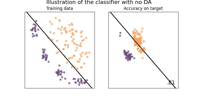
Illustration of the Density Reweighting method

This method is trying to compute the optimal weights as a ratio of two probability functions, by default, it is the ratio of two kernel densities estimations.

# We define our classifier, `clf` is a da pipeline
clf = DensityReweight(
    base_estimator=base_classifier,
    weight_estimator=KernelDensity(bandwidth=0.5),
)
clf.fit(X, y, sample_domain=sample_domain)

# We get the weights:

# we first get the adapter which is estimating the weights
weight_estimator = clf[0].get_estimator()
idx = extract_source_indices(sample_domain)
weights = weight_estimator.compute_weights(X, sample_domain=sample_domain)[idx]

plot_weights_and_classifier(clf, weights=weights, name="Density Reweighting")

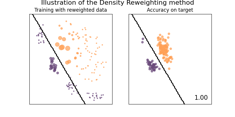
Illustration of the Gaussian reweighting method

This method tries to approximate the optimal weights by assuming that the data are normally distributed, and thus approximating the probability functions for both source and target set, and setting the weight to be the ratio of the two.

See [1] for details.

[1]

Hidetoshi Shimodaira. Improving predictive inference under covariate shift by weighting the log-likelihood function. In Journal of Statistical Planning and Inference, 2000.

# We define our classifier, `clf` is a da pipeline
clf = GaussianReweight(base_classifier)
clf.fit(X, y, sample_domain=sample_domain)
# We get the weights
weight_estimator = clf[0].get_estimator()
idx = extract_source_indices(sample_domain)
weights = weight_estimator.compute_weights(X, sample_domain=sample_domain)[idx]

plot_weights_and_classifier(clf, weights=weights, name="Gaussian Reweighting")

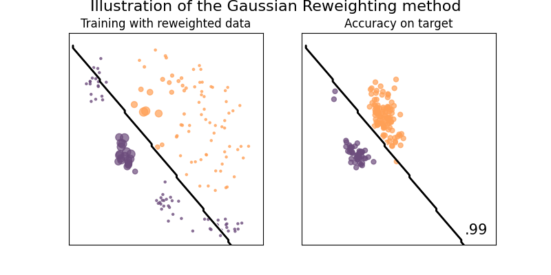
Illustration of the Discr. reweighting method

This estimator derive a class of predictive densities by weighting the source samples when trying to maximize the log-likelihood function. Such approach is effective in cases of covariate shift.

See [1] for details.

[1]

Hidetoshi Shimodaira. Improving predictive inference under covariate shift by weighting the log-likelihood function. In Journal of Statistical Planning and Inference, 2000.

# We define our classifier, `clf` is a da pipeline
clf = DiscriminatorReweight(base_classifier)
clf.fit(X, y, sample_domain=sample_domain)

# We get the weights:

# we first get the adapter which is estimating the weights
weight_estimator = clf[0].get_estimator()
idx = extract_source_indices(sample_domain)
weights = weight_estimator.compute_weights(X, sample_domain=sample_domain)[idx]

plot_weights_and_classifier(clf, weights=weights, name="Discr. Reweighting")

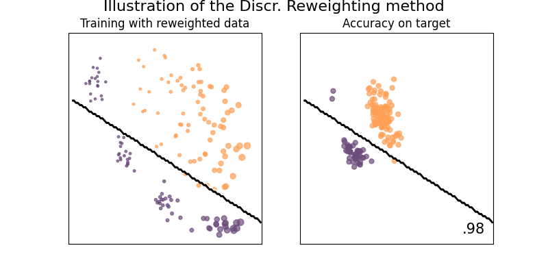
Illustration of the KLIEPReweight method

The idea of KLIEPReweight is to find an importance estimate \(w(x)\) such that the Kullback-Leibler (KL) divergence between the source input density \(p_{source}(x)\) to its estimate \(p_{target}(x) = w(x)p_{source}(x)\) is minimized.

See [3] for details.

[3]

Masashi Sugiyama et. al. Direct Importance Estimation with Model Selection and Its Application to Covariate Shift Adaptation. In NeurIPS, 2007.

# We define our classifier, `clf` is a da pipeline
clf = KLIEPReweight(
    LogisticRegression().set_fit_request(sample_weight=True), gamma=[1, 0.1, 0.001]
)
clf.fit(X, y, sample_domain=sample_domain)

# We get the weights:

# we first get the adapter which is estimating the weights
weight_estimator = clf[0].get_estimator()
idx = extract_source_indices(sample_domain)
weights = weight_estimator.compute_weights(X, sample_domain=sample_domain)[idx]

plot_weights_and_classifier(clf, weights=weights, name="KLIEPReweight")

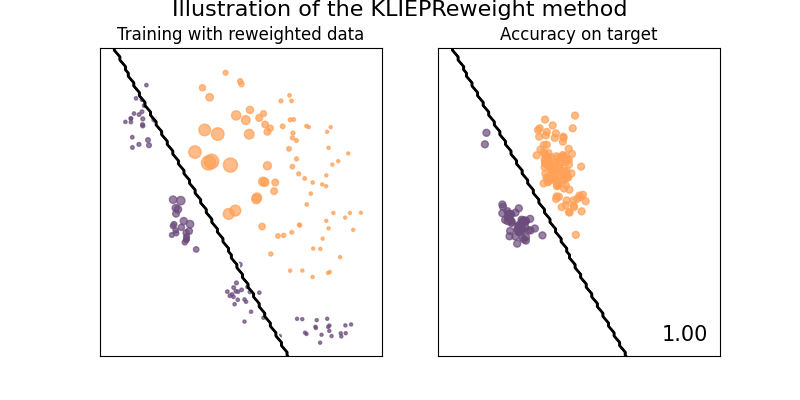
Illustration of the Nearest Neighbor reweighting method

This method estimate weight of a point in the source dataset by counting the number of points in the target set that are closer to it than any other points from the source dataset.

See [24] for details.

[24]

Loog, M. (2012). Nearest neighbor-based importance weighting. In 2012 IEEE International Workshop on Machine Learning for Signal Processing, pages 1–6. IEEE

# We define our classifier, `clf` is a da pipeline
clf = NearestNeighborReweight(base_classifier, laplace_smoothing=True)
clf.fit(X, y, sample_domain=sample_domain)

# We get the weights:

# we first get the adapter which is estimating the weights
weight_estimator = clf[0].get_estimator()
idx = extract_source_indices(sample_domain)
weights = weight_estimator.compute_weights(X, sample_domain=sample_domain)[idx]

plot_weights_and_classifier(clf, weights=weights, name="1NN Reweighting")

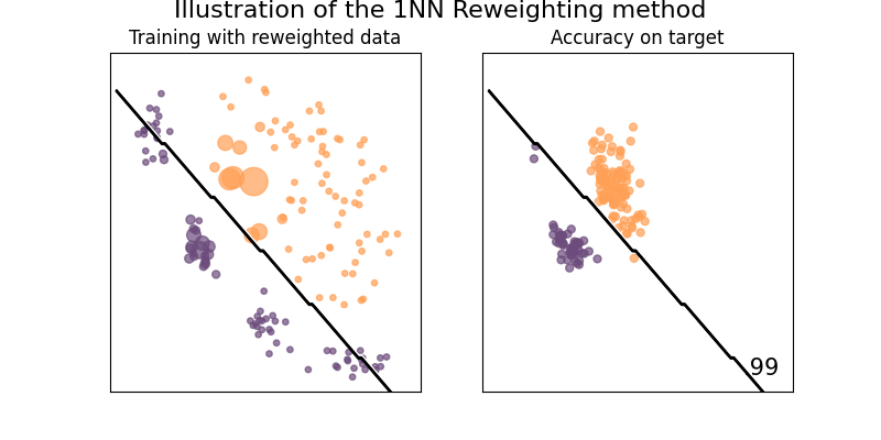
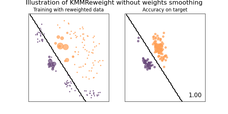
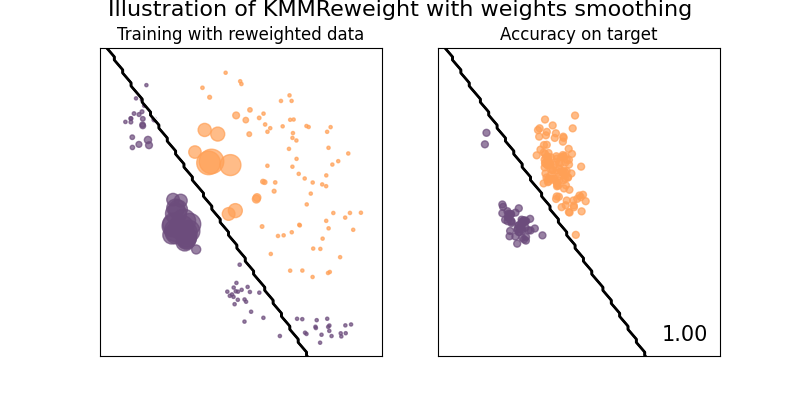
Illustration of the Kernel Mean Matching method

This example illustrates the use of KMMReweight method [6] to correct covariate-shift. This methods works without any estimation of the assumption, by matching distribution between training and testing sets in feature space.

See [25] for details.

[25]

J. Huang, A. Gretton, K. Borgwardt, B. Schölkopf and A. J. Smola. Correcting sample selection bias by unlabeled data. In NIPS, 2007.

# We define our classifier, `clf` is a da pipeline
clf = KMMReweight(base_classifier, gamma=10.0, max_iter=1000, smooth_weights=False)
clf.fit(X, y, sample_domain=sample_domain)

# We get the weights:

# we first get the adapter which is estimating the weights
weight_estimator = clf[0].get_estimator()
idx = extract_source_indices(sample_domain)
weights = weight_estimator.compute_weights(X, sample_domain=sample_domain)[idx]

plot_weights_and_classifier(
    clf,
    weights=weights,
    name="Kernel Mean Matching",
    suptitle="Illustration of KMMReweight without weights smoothing",
)

# We define our classifier, `clf` is a da pipeline
clf = KMMReweight(base_classifier, gamma=10.0, max_iter=1000, smooth_weights=True)
clf.fit(X, y, sample_domain=sample_domain)

# We get the weights:

# we first get the adapter which is estimating the weights
weight_estimator = clf[0].get_estimator()
idx = extract_source_indices(sample_domain)
weights = weight_estimator.compute_weights(X, sample_domain=sample_domain)[idx]

plot_weights_and_classifier(
    clf,
    weights=weights,
    name="Kernel Mean Matching",
    suptitle="Illustration of KMMReweight with weights smoothing",
)

# We define our classifier, `clf` is a da pipeline
clf = KMMReweight(
    base_classifier,
    gamma=10.0,
    max_iter=1000,
    smooth_weights=True,
    solver="frank-wolfe",
)
clf.fit(X, y, sample_domain=sample_domain)

# We get the weights:

# we first get the adapter which is estimating the weights
weight_estimator = clf[0].get_estimator()
idx = extract_source_indices(sample_domain)
weights = weight_estimator.compute_weights(X, sample_domain=sample_domain)[idx]

plot_weights_and_classifier(
    clf,
    weights=weights,
    name="Kernel Mean Matching",
    suptitle="Illustration of KMMReweight with Frank-Wolfe solver",
)

• 
• 
• 

Comparison of score between reweighting methods:

def print_scores_as_table(scores):
    max_len = max(len(k) for k in scores.keys())
    for k, v in scores.items():
        print(f"{k}{' '*(max_len - len(k))} | ", end="")
        print(f"{v*100}{' '*(6-len(str(v*100)))}%")


print_scores_as_table(scores_dict)

plt.show()

Without DA           | 80.625%
Density Reweighting  | 100.0 %
Gaussian Reweighting | 99.375%
Discr. Reweighting   | 98.125%
KLIEPReweight        | 100.0 %
1NN Reweighting      | 99.375%
Kernel Mean Matching | 100.0 %