Subspace method example on subspace shift dataset

An example of the subspace methods on a dataset subject to subspace shift

# Author:   Ruben Bueno <ruben.bueno@polytechnique.edu>
#           Antoine Collas <contact@antoinecollas.fr>
#           Oleksii Kachaiev <kachayev@gmail.com>
#
# License: BSD 3-Clause
# sphinx_gallery_thumbnail_number = 4

import matplotlib.pyplot as plt
import numpy as np
from matplotlib.colors import ListedColormap
from sklearn.inspection import DecisionBoundaryDisplay
from sklearn.svm import SVC

from skada import (
    SubspaceAlignment,
    TransferComponentAnalysis,
    TransferJointMatching,
    TransferSubspaceLearning,
    source_target_split,
)
from skada.datasets import make_shifted_datasets

The subspaces methods

Supspace methods are used in unsupervised domain adaptation. In this case, we have labeled data for the source domain but not for the target domain. The goal of subspace methods is to project data from a d-dimensional space into a lower-dimensional space with d' < d. Subspace methods are particularly effective when dealing with subspace shift, where the source and target data have the same distributions when projected onto a subspace.

# The Subspace methods implemented and illustrated are the following:
#   * :ref:`Subspace Alignment<Illustration of the Subspace Alignment method>`
#   * :ref:`Transfer Component Analysis<Illustration of the Transfer Component
#     Analysis method>`
#   * :ref:`Transfer Joint Matching<Illustration of the Transfer Joint Matching method>`


base_classifier = SVC()

print(f"Will be using {base_classifier} as base classifier", end="\n\n")

Will be using SVC() as base classifier

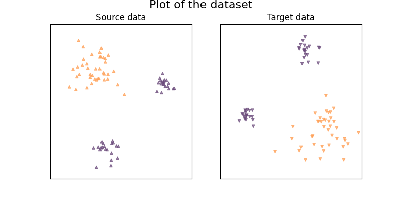
We generate our 2D dataset with 2 classes

We generate a simple 2D dataset with subspace shift.

RANDOM_SEED = 42

dataset = make_shifted_datasets(
    n_samples_source=20,
    n_samples_target=20,
    noise=0.1,
    random_state=RANDOM_SEED,
    shift="subspace",
    return_dataset=True,
)

X_train, y_train, sample_domain_train = dataset.pack_train(
    as_sources=["s"],
    as_targets=["t"],
)
X, y, sample_domain = dataset.pack(
    as_sources=["s"],
    as_targets=["t"],
    train=False,
)
Xs, Xt, ys, yt = source_target_split(X, y, sample_domain=sample_domain)

Plot of the dataset:

x_min, x_max = -2.4, 2.4
y_min, y_max = -2.4, 2.4
target_marker = "v"
source_marker = "^"

figsize = (8, 4)
figure, axes = plt.subplots(1, 2, figsize=figsize)

cm = plt.cm.RdBu
colormap = ListedColormap(["#FFA056", "#6C4C7C"])
ax = axes[0]
ax.set_title("Source data")
# Plot the source points:
ax.scatter(
    Xs[:, 0], Xs[:, 1], c=ys, cmap=colormap, alpha=0.7, s=[15], marker=source_marker
)

ax.set_xticks(()), ax.set_yticks(())
ax.set_xlim(x_min, x_max), ax.set_ylim(y_min, y_max)

ax = axes[1]

ax.set_title("Target data")
# Plot the target points:
ax.scatter(
    Xt[:, 0], Xt[:, 1], c=yt, cmap=colormap, alpha=0.7, s=[15], marker=target_marker
)
figure.suptitle("Plot of the dataset", fontsize=16, y=1)
ax.set_xticks(()), ax.set_yticks(())
ax.set_xlim(x_min, x_max), ax.set_ylim(y_min, y_max)

((-2.4, 2.4), (-2.4, 2.4))

Illustration of the problem with no domain adaptation

When not using domain adaptation, the classifier won't train on data that is distributed as the target sample domain, it will thus not be performing optimaly.

# We create a dict to store scores:
scores_dict = {}


def plot_subspace_and_classifier(
    clf,
    name="Without DA",
    suptitle=None,
):
    size = 16

    if suptitle is None:
        suptitle = f"Illustration of the {name} method"
    figure, axes = plt.subplots(1, 3, figsize=(figsize[0] * 1.5, figsize[1]))
    ax = axes[2]
    score = clf.score(Xt, yt)
    DecisionBoundaryDisplay.from_estimator(
        clf,
        Xs,
        cmap=colormap,
        alpha=0.1,
        ax=ax,
        eps=0.5,
        response_method="predict",
    )

    # Plot the target points:
    ax.scatter(
        Xt[:, 0], Xt[:, 1], c=yt, cmap=colormap, alpha=0.7, s=[15], marker=target_marker
    )

    ax.set_xticks(()), ax.set_yticks(())
    ax.set_xlim(x_min, x_max), ax.set_ylim(y_min, y_max)
    ax.set_title("Accuracy on target", fontsize=12)
    ax.text(
        x_max - 0.3,
        y_min + 0.3,
        ("%.2f" % score).lstrip("0"),
        size=15,
        horizontalalignment="right",
    )
    scores_dict[name] = score
    if name != "Without DA":
        subspace_estimator = clf.steps[-2][1].get_estimator()
        clf_on_subspace = clf.steps[-1][1].get_estimator()

        ax = axes[0]

        # Plot the source points:
        Xs_subspace = subspace_estimator.transform(
            Xs,
            # mark all samples as sources
            sample_domain=np.ones(Xs.shape[0]),
            allow_source=True,
        )
        Xt_subspace = subspace_estimator.transform(Xt)
        ax.scatter(
            Xs_subspace,
            [1] * Xs.shape[0],
            c=ys,
            cmap=colormap,
            alpha=0.5,
            s=size,
            marker=source_marker,
        )
        ax.scatter(
            Xt_subspace,
            [-1] * Xt.shape[0],
            c=yt,
            cmap=colormap,
            alpha=0.5,
            s=size,
            marker=target_marker,
        )

        ax.set_xticks(()), ax.set_yticks(())
        ax.set_ylim(-50, 50)
        ax.set_title("Full dataset projected on the subspace", fontsize=12)

        ax = axes[1]
        Xt_adapted = subspace_estimator.transform(Xt)
        ax.scatter(
            Xt_adapted,
            [0] * Xt.shape[0],
            c=yt,
            cmap=colormap,
            alpha=0.5,
            s=size,
            marker=target_marker,
        )
        m, M = min(Xt_adapted), max(Xt_adapted)
        x_ = list(np.linspace(m - abs(m) / 4, M + abs(M) / 4, 100).reshape(-1, 1))
        y_ = list(clf_on_subspace.predict(x_))
        ax.scatter(
            x_ * 100,
            [j // 100 - 50 for j in range(100 * 100)],
            c=y_ * 100,
            cmap=colormap,
            alpha=0.02,
            s=size,
        )
        ax.set_ylim(-50, 50)
        ax.set_title("Accuracy on target projected on the subspace", fontsize=12)
    else:
        ax = axes[0]
        ax.scatter(
            Xs[:, 0],
            Xs[:, 1],
            c=ys,
            cmap=colormap,
            alpha=0.5,
            s=size,
            marker=source_marker,
        )
        ax.scatter(
            Xt[:, 0],
            Xt[:, 1],
            c=yt,
            cmap=colormap,
            alpha=0.5,
            s=size,
            marker=target_marker,
        )

        ax.set_xticks(()), ax.set_yticks(())
        ax.set_xlim(x_min, x_max), ax.set_ylim(y_min, y_max)
        ax.set_title("Full dataset", fontsize=12)

        ax = axes[1]
        score = clf.score(Xs, ys)
        DecisionBoundaryDisplay.from_estimator(
            clf,
            Xs,
            cmap=colormap,
            alpha=0.1,
            ax=ax,
            eps=0.5,
            response_method="predict",
        )

        # Plot the source points:
        ax.scatter(
            Xs[:, 0],
            Xs[:, 1],
            c=ys,
            cmap=colormap,
            alpha=0.7,
            s=[15],
            marker=source_marker,
        )

        ax.set_xticks(()), ax.set_yticks(())
        ax.set_xlim(x_min, x_max), ax.set_ylim(y_min, y_max)
        ax.set_title("Accuracy on source", fontsize=12)
        ax.text(
            x_max - 0.3,
            y_min + 0.3,
            ("%.2f" % score).lstrip("0"),
            size=15,
            horizontalalignment="right",
        )

    figure.suptitle(suptitle, fontsize=16, y=1)
    figure.tight_layout()


clf = base_classifier
clf.fit(Xs, ys)
plot_subspace_and_classifier(
    base_classifier, "Without DA", suptitle="Illustration of the classifier with no DA"
)

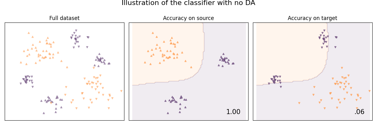
Illustration of the Subspace Alignment method

As we assume that the source and target domains are represented by subspaces described by eigenvectors; This method seeks a domain adaptation solution by learning a mapping function which aligns the source subspace with the target one.

See [8] for details:

[8]

Basura Fernando et. al. Unsupervised Visual Domain Adaptation Using Subspace Alignment. In IEEE International Conference on Computer Vision, 2013.

clf = SubspaceAlignment(base_classifier, n_components=1)
clf.fit(X_train, y_train, sample_domain=sample_domain_train)
plot_subspace_and_classifier(clf, "Subspace Alignment")

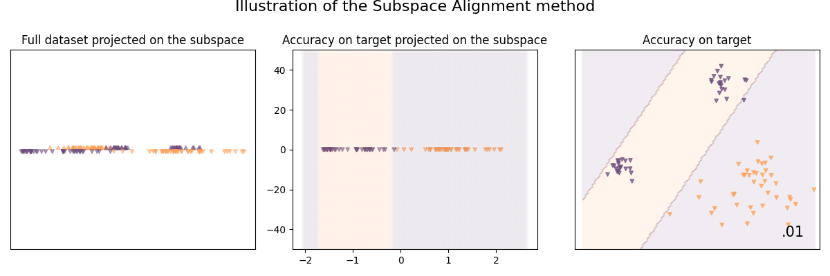
Illustration of the Transfer Component Analysis method

The goal of Transfer Component Analysis (TCA) is to learn some transfer components across domains in a reproducing kernel Hilbert space using Maximum Mean Discrepancy (MMD)

See [9] for details:

[9]

Sinno Jialin Pan et. al. Domain Adaptation via Transfer Component Analysis. In IEEE Transactions on Neural Networks, 2011.

clf = TransferComponentAnalysis(base_classifier, n_components=1, mu=2)
clf.fit(X_train, y_train, sample_domain=sample_domain_train)
plot_subspace_and_classifier(clf, "TCA")

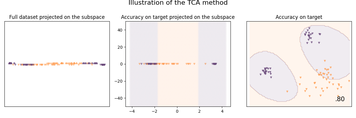
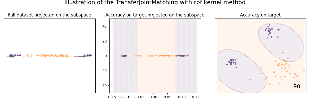
Illustration of the Transfer Joint Matching method

In most of the previous works, we explored two learning strategies independently for domain adaptation: feature matching and instance reweighting. Transfer Joint Matching (TJM) aims to use both, by adding a constant to tradeoff between the two.

See [26] for details:

[26]

Long et al., 2014] Long, M., Wang, J., Ding, G., Sun, J., and Yu, P. (2014). Transfer joint matching for unsupervised domain adaptation. In IEEE Conference on Computer Vision and Pattern Recognition (CVPR), pages 1410–1417.

clf = TransferJointMatching(base_classifier, tradeoff=0.1, n_components=1)
clf.fit(X_train, y_train, sample_domain=sample_domain_train)
plot_subspace_and_classifier(
    clf,
    "TransferJointMatching with rbf kernel",
)

/home/circleci/project/skada/_subspace.py:603: UserWarning: The solution of the generalized eigenvalue problem is not accurate.
  warnings.warn(

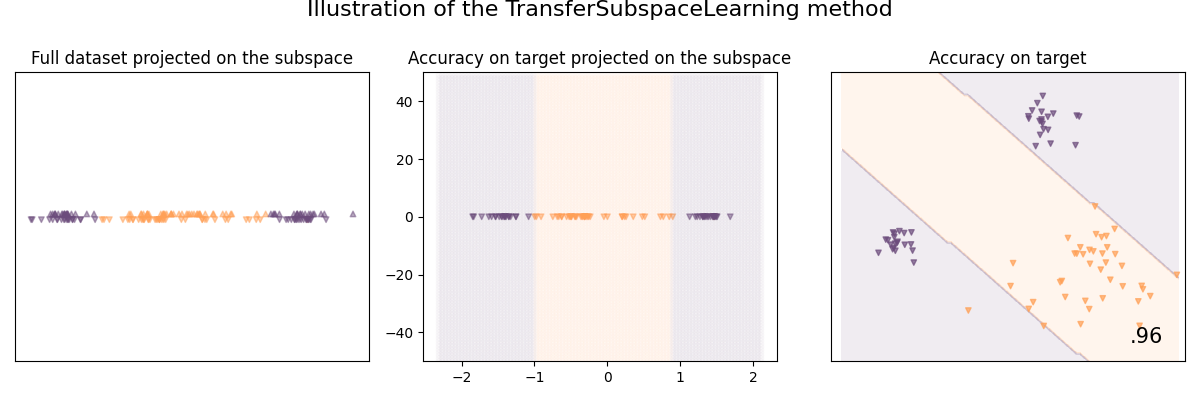
Illustration of the Transfer Subspace Learning method

Transfer Subspace Learning (TSL) is a method that aims to learn a subspace using classical loss functions (e.g. PCA, Fisher LDA) but regularized so that the source and target data have the same distribution once projected on the subspace.

See [27] for details:

[27]

[Si et al., 2010] Si, S., Tao, D. and Geng, B. Bregman Divergence-Based Regularization for Transfer Subspace Learning. In IEEE Transactions on Knowledge and Data Engineering. pages 929-942

clf = TransferSubspaceLearning(base_classifier, n_components=1)
clf.fit(X, y, sample_domain=sample_domain)
plot_subspace_and_classifier(clf, "TransferSubspaceLearning")

/home/circleci/project/skada/utils.py:920: UserWarning: To copy construct from a tensor, it is recommended to use sourceTensor.clone().detach() or sourceTensor.clone().detach().requires_grad_(True), rather than torch.tensor(sourceTensor).
  x0 = [torch.tensor(x, requires_grad=True, dtype=torch.float64) for x in x0]

Comparison of score between subspace methods:

def print_scores_as_table(scores):
    max_len = max(len(k) for k in scores.keys())
    for k, v in scores.items():
        print(f"{k}{' '*(max_len - len(k))} | ", end="")
        print(f"{v*100}{' '*(6-len(str(v*100)))}%")


print_scores_as_table(scores_dict)

plt.show()

Without DA                            | 6.25  %
Subspace Alignment                    | 1.25  %
TCA                                   | 80.0  %
TransferJointMatching with rbf kernel | 90.0  %
TransferSubspaceLearning              | 96.25 %