Note
Go to the end to download the full example code.
Label Propagation methods
This example shows how to use how to use label propagation methods to perform domain adaptation. This is done by propagating labels from the source domain to the target domain using the OT plan. This was proposed originally in [28] for semi-supervised learning but can be used for DA.
We illustrate the method on a simple regression and classification conditional shift dataset. We train a simple Kernel Ridge Regression (KRR) and Logistic Regression on the source domain and evaluate their performance on the source and target domain. We then train the same models with the label propagation method and evaluate their performance on the source and target domain.
# Author: Remi Flamary
#
# License: BSD 3-Clause
# sphinx_gallery_thumbnail_number = 4
import matplotlib.pyplot as plt
import numpy as np
from sklearn.kernel_ridge import KernelRidge
from sklearn.linear_model import LogisticRegression
from sklearn.metrics import mean_squared_error
from sklearn.svm import SVC

from skada import (
    JCPOTLabelPropAdapter,
    OTLabelPropAdapter,
    make_da_pipeline,
    source_target_split,
)
from skada.datasets import make_shifted_datasets
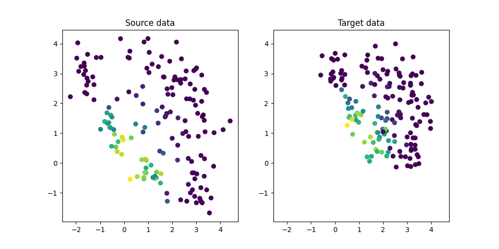
Generate conditional shift regression dataset and plot it
We generate a simple 2D conditional shift dataset.
X, y, sample_domain = make_shifted_datasets(
    n_samples_source=20,
    n_samples_target=20,
    shift="conditional_shift",
    noise=0.3,
    label="regression",
    random_state=42,
)

y = (y - y.mean()) / y.std()

Xs, Xt, ys, yt = source_target_split(X, y, sample_domain=sample_domain)


plt.figure(1, (10, 5))
plt.subplot(1, 2, 1)
plt.scatter(Xs[:, 0], Xs[:, 1], c=ys, label="Source")
plt.title("Source data")
ax = plt.axis()

plt.subplot(1, 2, 2)
plt.scatter(Xt[:, 0], Xt[:, 1], c=yt, label="Target")
plt.title("Target data")
plt.axis(ax)
(np.float64(-2.570318895725525), np.float64(4.744989537549497), np.float64(-1.9610814126500358), np.float64(4.45933195939893))
Train a regressor on source data
We train a simple Kernel Ridge Regression (KRR) on the source domain and evaluate its performance on the source and target domain. Performance is much lower on the target domain due to the shift. We also plot the decision boundary learned by the KRR.
clf = KernelRidge(kernel="rbf", alpha=0.5)
clf.fit(Xs, ys)

# Compute accuracy on source and target
ys_pred = clf.predict(Xs)
yt_pred = clf.predict(Xt)

mse_s = mean_squared_error(ys, ys_pred)
mse_t = mean_squared_error(yt, yt_pred)

print(f"MSE on source: {mse_s:.2f}")
print(f"MSE on target: {mse_t:.2f}")

XX, YY = np.meshgrid(np.linspace(ax[0], ax[1], 100), np.linspace(ax[2], ax[3], 100))
Z = clf.predict(np.c_[XX.ravel(), YY.ravel()]).reshape(XX.shape)


plt.figure(2, (10, 5))
plt.subplot(1, 2, 1)
plt.scatter(Xs[:, 0], Xs[:, 1], c=ys, label="Prediction")
plt.imshow(Z, extent=(ax[0], ax[1], ax[2], ax[3]), origin="lower", alpha=0.5)
plt.title(f"KRR Prediction on source (MSE={mse_s:.2f})")
plt.axis(ax)

plt.subplot(1, 2, 2)
plt.scatter(Xt[:, 0], Xt[:, 1], c=yt, label="Prediction")
plt.imshow(Z, extent=(ax[0], ax[1], ax[2], ax[3]), origin="lower", alpha=0.5)
plt.title(f"KRR Prediction on target (MSE={mse_t:.2f})")
plt.axis(ax)
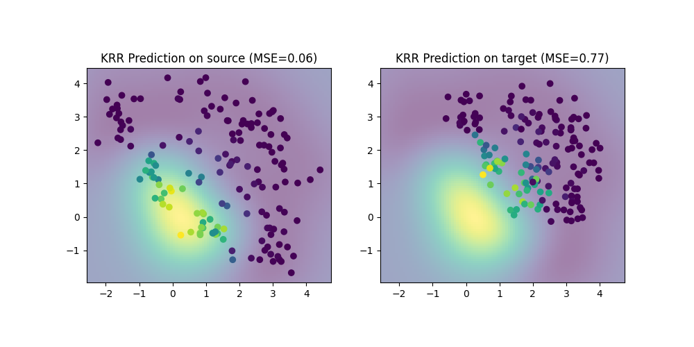
MSE on source: 0.06
MSE on target: 0.77

(np.float64(-2.570318895725525), np.float64(4.744989537549497), np.float64(-1.9610814126500358), np.float64(4.45933195939893))
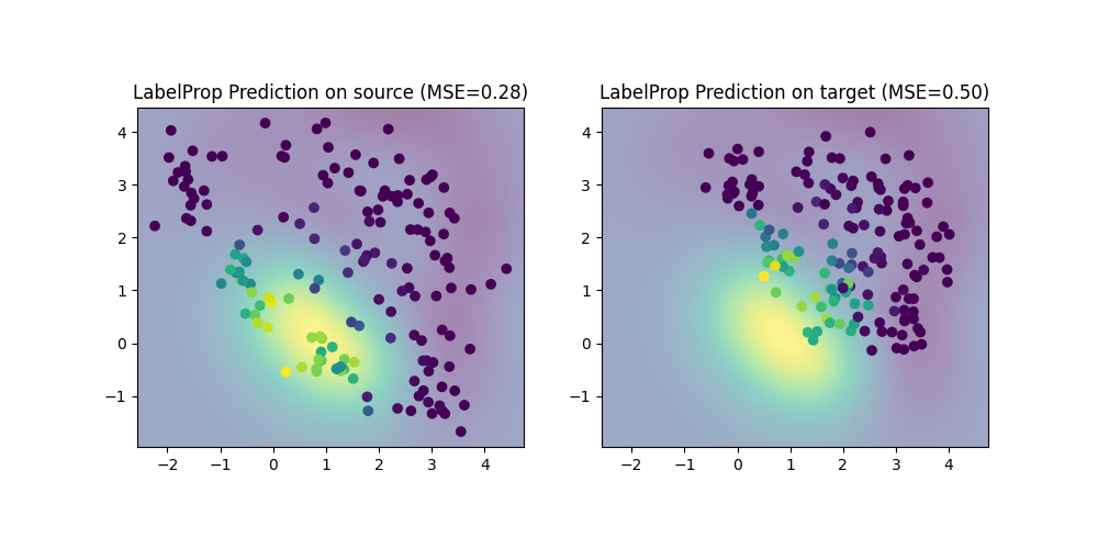
Train the full Labe Propagation model
clf = make_da_pipeline(OTLabelPropAdapter(), KernelRidge(kernel="rbf", alpha=0.5))
clf.fit(X, y, sample_domain=sample_domain)

ys_pred = clf.predict(Xs)
yt_pred = clf.predict(Xt)

mse_s = mean_squared_error(ys, ys_pred)
mse_t = mean_squared_error(yt, yt_pred)

Zjdot = clf.predict(np.c_[XX.ravel(), YY.ravel()]).reshape(XX.shape)

print(f"LabelProp MSE on source: {mse_s:.2f}")
print(f"LabelProp MSE on target: {mse_t:.2f}")

plt.figure(3, (10, 5))
plt.subplot(1, 2, 1)
plt.scatter(Xs[:, 0], Xs[:, 1], c=ys, label="Prediction")
plt.imshow(Zjdot, extent=(ax[0], ax[1], ax[2], ax[3]), origin="lower", alpha=0.5)
plt.title(f"LabelProp Prediction on source (MSE={mse_s:.2f})")
plt.axis(ax)

plt.subplot(1, 2, 2)
plt.scatter(Xt[:, 0], Xt[:, 1], c=yt, label="Prediction")
plt.imshow(Zjdot, extent=(ax[0], ax[1], ax[2], ax[3]), origin="lower", alpha=0.5)
plt.title(f"LabelProp Prediction on target (MSE={mse_t:.2f})")
plt.axis(ax)
/home/circleci/.local/lib/python3.10/site-packages/ot/lp/_network_simplex.py:520: UserWarning: numItermax reached before optimality. Try to increase numItermax.
  result_code_string = check_result(result_code)
LabelProp MSE on source: 0.28
LabelProp MSE on target: 0.50

(np.float64(-2.570318895725525), np.float64(4.744989537549497), np.float64(-1.9610814126500358), np.float64(4.45933195939893))
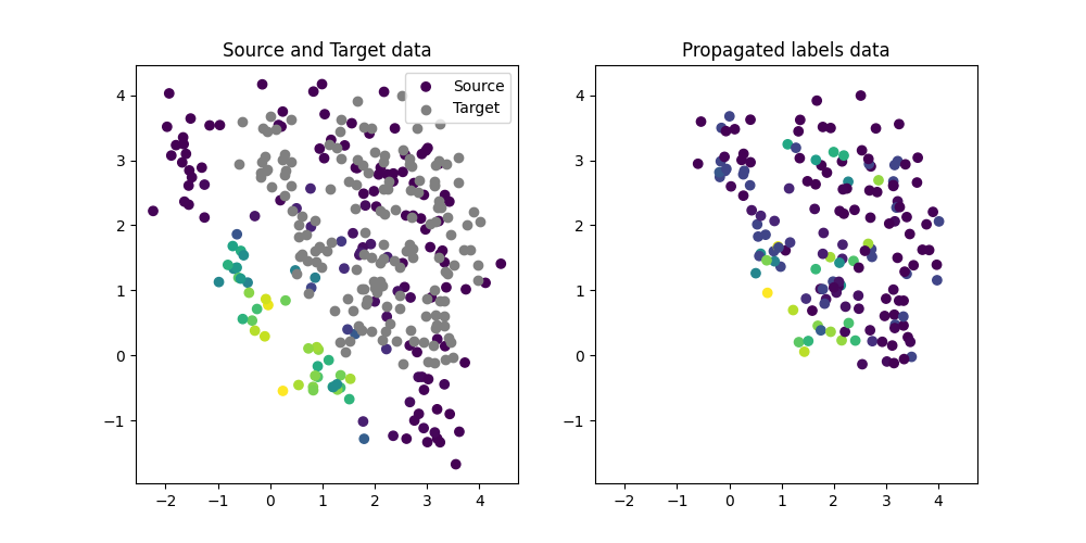
Illustration of the propagated labels
We illustrate the propagated labels on the target domain. We can see that the labels are propagated from the source domain to the target domain.
lp = OTLabelPropAdapter()

yh = lp.fit_transform(X, y, sample_domain=sample_domain)[1]

yht = yh[sample_domain < 0]  #

plt.figure(1, (10, 5))
plt.subplot(1, 2, 1)
plt.scatter(Xs[:, 0], Xs[:, 1], c=ys, label="Source")
plt.scatter(Xt[:, 0], Xt[:, 1], c="gray", label="Target")
plt.legend()

plt.title("Source and Target data")
ax = plt.axis()

plt.subplot(1, 2, 2)
plt.scatter(Xt[:, 0], Xt[:, 1], c=yht, label="Target")


plt.title("Propagated labels data")
plt.axis(ax)
/home/circleci/.local/lib/python3.10/site-packages/ot/lp/_network_simplex.py:520: UserWarning: numItermax reached before optimality. Try to increase numItermax.
  result_code_string = check_result(result_code)

(np.float64(-2.570318895725525), np.float64(4.744989537549497), np.float64(-1.9610814126500358), np.float64(4.45933195939893))
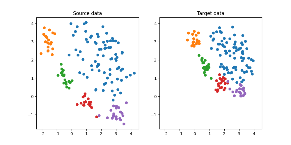
Generate conditional shift classification dataset and plot it
We generate a simple 2D conditional shift dataset.
X, y, sample_domain = make_shifted_datasets(
    n_samples_source=20,
    n_samples_target=20,
    shift="conditional_shift",
    noise=0.2,
    label="multiclass",
    random_state=42,
)


Xs, Xt, ys, yt = source_target_split(X, y, sample_domain=sample_domain)


plt.figure(5, (10, 5))
plt.subplot(1, 2, 1)
plt.scatter(Xs[:, 0], Xs[:, 1], c=ys, cmap="tab10", vmax=9, label="Source")
plt.title("Source data")
ax = plt.axis()

plt.subplot(1, 2, 2)
plt.scatter(Xt[:, 0], Xt[:, 1], c=yt, cmap="tab10", vmax=9, label="Target")
plt.title("Target data")
plt.axis(ax)
(np.float64(-2.3676169789533272), np.float64(4.53817259426296), np.float64(-1.7964573229829714), np.float64(4.336863129384494))
Train a classifier on source data
We train a simple SVC classifier on the source domain and evaluate its performance on the source and target domain. Performance is much lower on the target domain due to the shift. We also plot the decision boundary
clf = LogisticRegression()
clf.fit(Xs, ys)

# Compute accuracy on source and target
ys_pred = clf.predict(Xs)
yt_pred = clf.predict(Xt)

acc_s = (ys_pred == ys).mean()
acc_t = (yt_pred == yt).mean()

print(f"Accuracy on source: {acc_s:.2f}")
print(f"Accuracy on target: {acc_t:.2f}")

XX, YY = np.meshgrid(np.linspace(ax[0], ax[1], 100), np.linspace(ax[2], ax[3], 100))
Z = clf.predict(np.c_[XX.ravel(), YY.ravel()]).reshape(XX.shape)


plt.figure(6, (10, 5))
plt.subplot(1, 2, 1)
plt.scatter(Xs[:, 0], Xs[:, 1], c=ys, cmap="tab10", vmax=9, label="Prediction")
plt.imshow(
    Z,
    extent=(ax[0], ax[1], ax[2], ax[3]),
    origin="lower",
    alpha=0.5,
    cmap="tab10",
    vmax=9,
)
plt.title(f"LogReg Prediction on source (ACC={acc_s:.2f})")

plt.subplot(1, 2, 2)
plt.scatter(Xt[:, 0], Xt[:, 1], c=yt, cmap="tab10", vmax=9, label="Prediction")
plt.imshow(
    Z,
    extent=(ax[0], ax[1], ax[2], ax[3]),
    origin="lower",
    alpha=0.5,
    cmap="tab10",
    vmax=9,
)
plt.title(f"LogReg Prediction on target (ACC={acc_t:.2f})")
plt.axis(ax)
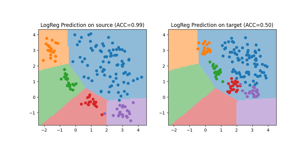
Accuracy on source: 0.99
Accuracy on target: 0.50

(np.float64(-2.3676169789533272), np.float64(4.53817259426296), np.float64(-1.7964573229829714), np.float64(4.336863129384494))
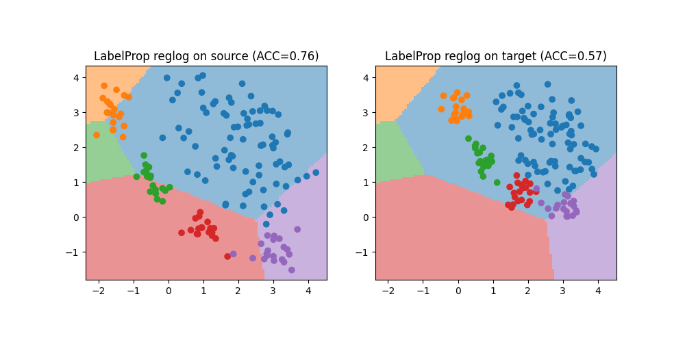
Train with LabelProp + classifier
clf = make_da_pipeline(OTLabelPropAdapter(), LogisticRegression())
clf.fit(X, y, sample_domain=sample_domain)


ys_pred = clf.predict(Xs)
yt_pred = clf.predict(Xt)

acc_s = (ys_pred == ys).mean()
acc_t = (yt_pred == yt).mean()

print(f"LabelProp Accuracy on source: {acc_s:.2f}")
print(f"LabelProp Accuracy on target: {acc_t:.2f}")

XX, YY = np.meshgrid(np.linspace(ax[0], ax[1], 100), np.linspace(ax[2], ax[3], 100))
Z = clf.predict(np.c_[XX.ravel(), YY.ravel()]).reshape(XX.shape)


plt.figure(7, (10, 5))
plt.subplot(1, 2, 1)
plt.scatter(Xs[:, 0], Xs[:, 1], c=ys, cmap="tab10", vmax=9, label="Prediction")
plt.imshow(
    Z,
    extent=(ax[0], ax[1], ax[2], ax[3]),
    origin="lower",
    alpha=0.5,
    cmap="tab10",
    vmax=9,
)
plt.title(f"LabelProp reglog on source (ACC={acc_s:.2f})")

plt.subplot(1, 2, 2)
plt.scatter(Xt[:, 0], Xt[:, 1], c=yt, cmap="tab10", vmax=9, label="Prediction")
plt.imshow(
    Z,
    extent=(ax[0], ax[1], ax[2], ax[3]),
    origin="lower",
    alpha=0.5,
    cmap="tab10",
    vmax=9,
)
plt.title(f"LabelProp reglog on target (ACC={acc_t:.2f})")
plt.axis(ax)
/home/circleci/.local/lib/python3.10/site-packages/ot/lp/_network_simplex.py:520: UserWarning: numItermax reached before optimality. Try to increase numItermax.
  result_code_string = check_result(result_code)
LabelProp Accuracy on source: 0.76
LabelProp Accuracy on target: 0.57

(np.float64(-2.3676169789533272), np.float64(4.53817259426296), np.float64(-1.7964573229829714), np.float64(4.336863129384494))
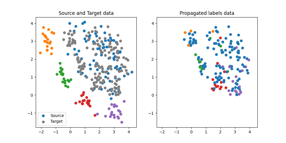
Illustration of the propagated labels
We illustrate the propagated labels on the target domain. We can see that the labels are propagated from the source domain to the target domain.
lp = OTLabelPropAdapter()

yh = lp.fit_transform(X, y, sample_domain=sample_domain)[1]

yht = yh[sample_domain < 0]

plt.figure(1, (10, 5))
plt.subplot(1, 2, 1)
plt.scatter(Xs[:, 0], Xs[:, 1], c=ys, cmap="tab10", vmax=9, label="Source")
plt.scatter(Xt[:, 0], Xt[:, 1], c="gray", label="Target")
plt.legend()
plt.title("Source and Target data")
ax = plt.axis()

plt.subplot(1, 2, 2)
plt.scatter(Xt[:, 0], Xt[:, 1], c=yht, cmap="tab10", vmax=9, label="Target")


plt.title("Propagated labels data")
plt.axis(ax)
/home/circleci/.local/lib/python3.10/site-packages/ot/lp/_network_simplex.py:520: UserWarning: numItermax reached before optimality. Try to increase numItermax.
  result_code_string = check_result(result_code)

(np.float64(-2.3676169789533272), np.float64(4.53817259426296), np.float64(-1.7964573229829714), np.float64(4.336863129384494))
Generate classification classification dataset and plot it
We generate a simple 2D target shift dataset.
X, y, sample_domain = make_shifted_datasets(
    n_samples_source=20,
    n_samples_target=20,
    shift="target_shift",
    noise=0.2,
    random_state=42,
)


Xs, Xt, ys, yt = source_target_split(X, y, sample_domain=sample_domain)


plt.figure(5, (10, 5))
plt.subplot(1, 2, 1)
plt.scatter(Xs[:, 0], Xs[:, 1], c=ys, cmap="tab10", vmax=9, label="Source")
plt.title("Source data")
ax = plt.axis()

plt.subplot(1, 2, 2)
plt.scatter(Xt[:, 0], Xt[:, 1], c=yt, cmap="tab10", vmax=9, label="Target")
plt.title("Target data")
plt.axis(ax)
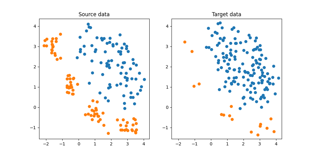
(np.float64(-2.4269298070320042), np.float64(4.352173719537829), np.float64(-1.5585726101363702), np.float64(4.367467726151268))
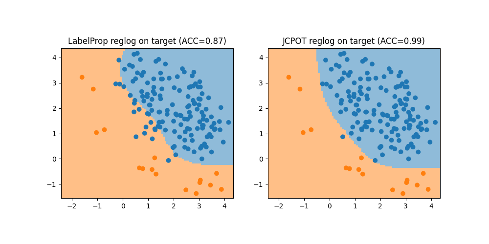
Train with LabelProp and JCPOT + classifier
On this target shift dataset, we can see that the label propagation method does not work well because it finds correspondences between the source and target samples with different classes. In this case JCPOT is more robust to this kind of shift because it estimates the class proportions in the target.
clf = make_da_pipeline(OTLabelPropAdapter(), SVC())
clf.fit(X, y, sample_domain=sample_domain)

clf_jcpot = make_da_pipeline(JCPOTLabelPropAdapter(reg=0.1), SVC())
clf_jcpot.fit(X, y, sample_domain=sample_domain)


yt_pred = clf.predict(Xt)
acc_t = (yt_pred == yt).mean()

print(f"LabelProp Accuracy on target: {acc_t:.2f}")


yt_pred = clf_jcpot.predict(Xt)
acc_s_jcpot = (yt_pred == yt).mean()

print(f"JCPOT Accuracy on target: {acc_s_jcpot:.2f}")

XX, YY = np.meshgrid(np.linspace(ax[0], ax[1], 100), np.linspace(ax[2], ax[3], 100))
Z = clf.predict(np.c_[XX.ravel(), YY.ravel()]).reshape(XX.shape)
Z_jcpot = clf_jcpot.predict(np.c_[XX.ravel(), YY.ravel()]).reshape(XX.shape)


plt.figure(7, (10, 5))


plt.subplot(1, 2, 1)
plt.scatter(Xt[:, 0], Xt[:, 1], c=yt, cmap="tab10", vmax=9, label="Prediction")
plt.imshow(
    Z,
    extent=(ax[0], ax[1], ax[2], ax[3]),
    origin="lower",
    alpha=0.5,
    cmap="tab10",
    vmax=9,
)
plt.title(f"LabelProp reglog on target (ACC={acc_t:.2f})")
plt.axis(ax)

plt.subplot(1, 2, 2)
plt.scatter(Xt[:, 0], Xt[:, 1], c=yt, cmap="tab10", vmax=9, label="Prediction")
plt.imshow(
    Z_jcpot,
    extent=(ax[0], ax[1], ax[2], ax[3]),
    origin="lower",
    alpha=0.5,
    cmap="tab10",
    vmax=9,
)
plt.title(f"JCPOT reglog on target (ACC={acc_s_jcpot:.2f})")
plt.axis(ax)
/home/circleci/.local/lib/python3.10/site-packages/ot/lp/_network_simplex.py:520: UserWarning: numItermax reached before optimality. Try to increase numItermax.
  result_code_string = check_result(result_code)
/home/circleci/.local/lib/python3.10/site-packages/ot/bregman/_barycenter.py:1048: UserWarning: Algorithm did not converge. You might want to increase the number of iterations `numItermax` or the regularization parameter `reg`.
  warnings.warn(
LabelProp Accuracy on target: 0.87
JCPOT Accuracy on target: 0.99

(np.float64(-2.4269298070320042), np.float64(4.352173719537829), np.float64(-1.5585726101363702), np.float64(4.367467726151268))
Total running time of the script: (0 minutes 2.302 seconds)